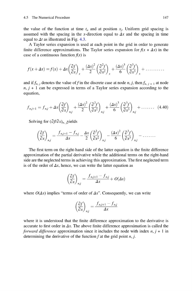
the value of the function at time t n and at position x j . Uniform grid spacing is
assumed with the spacing in the x-direction equal to Δx and the spacing in time
equal to Δt as illustrated in Fig. 4.3.
A Taylor series expansion is used at each point in the grid in order to generate
finite difference approximations. The Taylor series expansion for f(x + Δx) in the
case of a continuous function f(x) is
f x þ Δx
ð
Þ¼f x
ð Þ þ Δx
∂f
∂x
x
þ
Δx
ð Þ
2
2
∂
2 f
∂x 2
x
þ
Δx
ð Þ
3
6
∂
3 f
∂x 3
x
þ : . . . . . . . . .
and if f n, j denotes the value of f in the discrete case at node n, j, then f n, j + 1 at node
n, j + 1 can be expressed in terms of a Taylor series expansion according to the
equation,
f n,jþ1 ¼ f n,j þ Δx
∂f
∂x
n,j
þ
Δx
ð Þ
2
2
∂
2 f
∂x 2
n,j
þ
Δx
ð Þ
3
6
∂
3 f
∂x 3
n,j
þ : . . . . . . ð4:40Þ
Solving for (∂f/∂x) n, j yields
∂f
∂x
n,j
¼
f n,jþ1 À f n,j
Δx
À
Δx
2
∂
2 f
∂x 2
n,j
À
Δx
ð Þ
2
6
∂
3 f
∂x 3
n,j
À : . . . . . .
The first term on the right-hand side of the latter equation is the finite difference
approximation of the partial derivative while the additional terms on the right-hand
side are the neglected terms in achieving this approximation. The first neglected term
is of the order of Δx, hence, we can write the latter equation as
∂f
∂x
n,j
¼
f n,jþ1 À f n,j
Δx
þ O Δx
ð Þ
where O(Δx) implies “terms of order of Δx”. Consequently, we can write
∂f
∂x
n,j
¼
f n,jþ1 À f n,j
Δx
where it is understood that the finite difference approximation to the derivative is
accurate to first order in Δx. The above finite difference approximation is called the
forward difference approximation since it includes the node with index n, j + 1 in
determining the derivative of the function f at the grid point n, j.
4.5 The Numerical Procedure
147