

γp þ γ À 1
ð
Þq
½
∂υ
∂t
þ υ
∂p
∂t
¼ 0;
Energy
ð
Þ,
where q is given by,
q ¼ À
κΔx
ð
Þ
2
υ
∂u
∂x
∂u
∂x
: Artificial viscosity
ð
Þ
The derivatives in the above equations are replaced by a finite difference representation of these derivatives in order to obtain a numerical solution. In this
discretization process the functions (such as, pressure density etc.) have prescribed
values at only a finite number of discrete points in space and time, in contrast to a
continuous variation in these functions in the case of an analytical solution.
The highest-order derivatives that appear in the equations above are first-order
partial derivatives so that finite difference equations for first-order derivative are
required for the numerical procedure. Only a single spatial coordinate in addition to
the time t is required for the one-dimensional flow problems presented in this
chapter.
4.5.2 Finite Difference Expressions
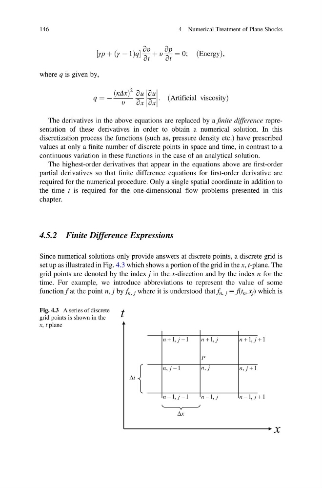
Since numerical solutions only provide answers at discrete points, a discrete grid is
set up as illustrated in Fig. 4.3 which shows a portion of the grid in the x, t-plane. The
grid points are denoted by the index j in the x-direction and by the index n for the
time. For example, we introduce abbreviations to represent the value of some
function f at the point n, j by f n, j where it is understood that f n, j f(t n , x j ) which is
Fig. 4.3 A series of discrete
grid points is shown in the
x, t plane
146
4 Numerical Treatment of Plane Shocks
ð
Þq
½
∂υ
∂t
þ υ
∂p
∂t
¼ 0;
Energy
ð
Þ,
where q is given by,
q ¼ À
κΔx
ð
Þ
2
υ
∂u
∂x
∂u
∂x
: Artificial viscosity
ð
Þ
The derivatives in the above equations are replaced by a finite difference representation of these derivatives in order to obtain a numerical solution. In this
discretization process the functions (such as, pressure density etc.) have prescribed
values at only a finite number of discrete points in space and time, in contrast to a
continuous variation in these functions in the case of an analytical solution.
The highest-order derivatives that appear in the equations above are first-order
partial derivatives so that finite difference equations for first-order derivative are
required for the numerical procedure. Only a single spatial coordinate in addition to
the time t is required for the one-dimensional flow problems presented in this
chapter.
4.5.2 Finite Difference Expressions
Since numerical solutions only provide answers at discrete points, a discrete grid is
set up as illustrated in Fig. 4.3 which shows a portion of the grid in the x, t-plane. The
grid points are denoted by the index j in the x-direction and by the index n for the
time. For example, we introduce abbreviations to represent the value of some
function f at the point n, j by f n, j where it is understood that f n, j f(t n , x j ) which is
Fig. 4.3 A series of discrete
grid points is shown in the
x, t plane
146
4 Numerical Treatment of Plane Shocks