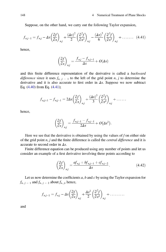
Suppose, on the other hand, we carry out the following Taylor expansion,
f n,jÀ1 ¼ f n,j À Δx
∂f
∂x
n,j
þ
Δx
ð Þ
2
2
∂
2 f
∂x 2
n,j
À
Δx
ð Þ
3
6
∂
3 f
∂x 3
n,j
þ : . . . . . . ð4:41Þ
hence,
∂f
∂x
n,j
¼
f n,j À f n,jÀ1
Δx
þ O Δx
ð Þ
and this finite difference representation of the derivative is called a backward
difference since it uses f n, j À 1 to the left of the grid point n, j to determine the
derivative and it is also accurate to first order in Δx. Suppose we now subtract
Eq. (4.40) from Eq. (4.41);
f n,jþ1 À f n,jÀ1 ¼ 2Δx
∂f
∂x
n,j
þ
Δx
ð Þ
3
3
∂
2 f
∂x 2
n,j
þ . . . . . .
hence,
∂f
∂x
n,j
¼
f n,jþ1 À f n,jÀ1
2Δx
þ O Δx
2
À Á :
Here we see that the derivative is obtained by using the values of f on either side
of the grid point n, j and the finite difference is called the central difference and it is
accurate to second order in Δx.
Finite difference equation can be produced using any number of points and let us
consider an example of a first derivative involving three points according to
∂f
∂x
n,j
¼
af n,j þ bf n,jÀ1 þ cf n,jÀ2
Δx
:
ð4:42Þ
Let us now determine the coefficients a, b and c by using the Taylor expansion for
f n, j À 1 and f n, j À 2 about f n, j , hence,
f n,jÀ1 ¼ f n,j À Δx
∂f
∂x
n,j
þ
Δx
2
2
∂
2 f
∂x 2
n,j
þ . . . . . . . . .
and
148
4 Numerical Treatment of Plane Shocks