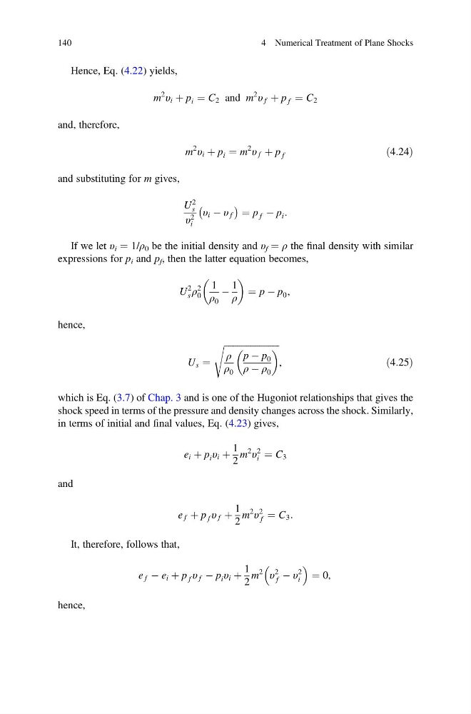
Hence, Eq. (4.22) yields,
m
2
υ i þ p i ¼ C 2 and m
2
υ f þ p f ¼ C 2
and, therefore,
m
2
υ i þ p i ¼ m
2
υ f þ p f
ð4:24Þ
and substituting for m gives,
U
2
s
υ 2
i
υ i À υ f
À
Á ¼ p f À p i :
If we let υ i ¼ 1/ρ 0 be the initial density and υ f ¼ ρ the final density with similar
expressions for p i and p f , then the latter equation becomes,
U
2
s ρ
2
0
1
ρ 0
À
1
ρ
¼ p À p 0 ,
hence,
U s ¼
ffiffiffiffiffiffiffiffiffiffiffiffiffiffiffiffiffiffiffiffiffiffiffiffiffi
ρ
ρ 0
p À p 0
ρ À ρ 0
s
,
ð4:25Þ
which is Eq. (3.7) of Chap. 3 and is one of the Hugoniot relationships that gives the
shock speed in terms of the pressure and density changes across the shock. Similarly,
in terms of initial and final values, Eq. (4.23) gives,
e i þ p i υ i þ
1
2
m
2
υ
2
i ¼ C 3
and
e f þ p f υ f þ
1
2
m
2
υ
2
f ¼ C 3 :
It, therefore, follows that,
e f À e i þ p f υ f À p i υ i þ
1
2
m
2
υ
2
f À υ
2
i
¼ 0,
hence,
140
4 Numerical Treatment of Plane Shocks