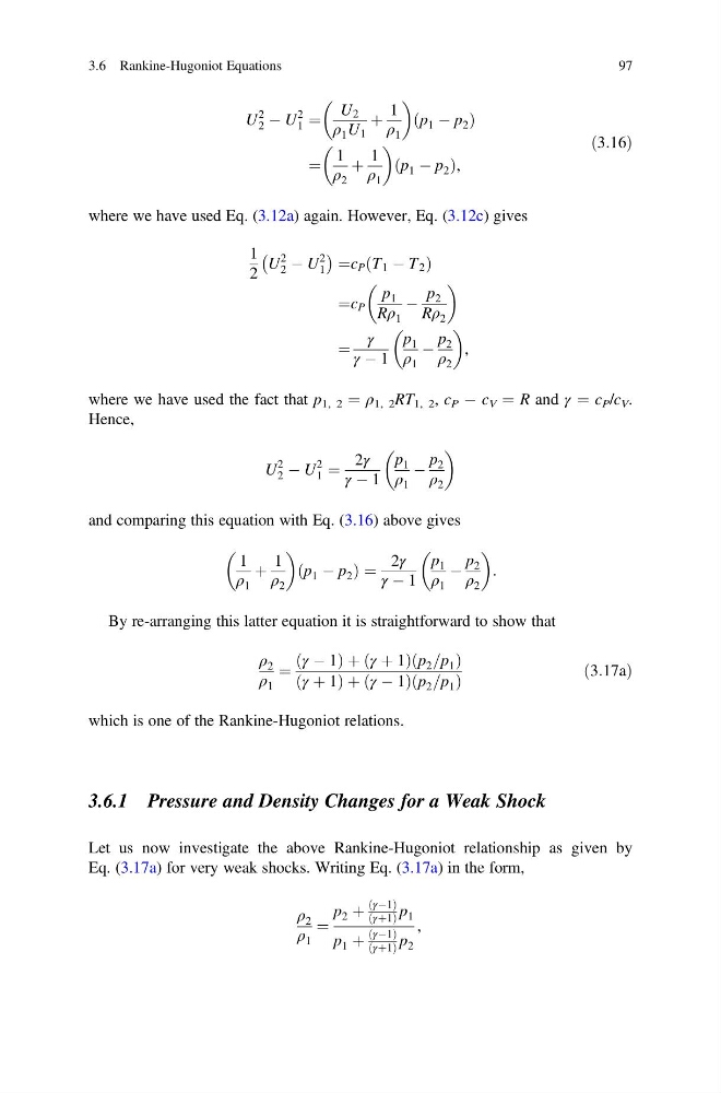
U
2
2 À U
2
1 ¼
U 2
ρ 1 U 1
þ
1
ρ 1
p 1 À p 2
ð
Þ
¼
1
ρ 2
þ
1
ρ 1
p 1 À p 2
ð
Þ ,
ð3:16Þ
where we have used Eq. (3.12a) again. However, Eq. (3.12c) gives
1
2
U
2
2 À U
2
1
À
Á ¼c P T 1 À T 2
ð
Þ
¼c P
p 1
Rρ 1
À
p 2
Rρ 2
¼
γ
γ À 1
p 1
ρ 1
À
p 2
ρ 2
,
where we have used the fact that p 1, 2 ¼ ρ 1, 2 RT 1, 2 , c P À c V ¼ R and γ ¼ c P /c V .
Hence,
U
2
2 À U
2
1 ¼
2γ
γ À 1
p 1
ρ 1
À
p 2
ρ 2
and comparing this equation with Eq. (3.16) above gives
1
ρ 1
þ
1
ρ 2
p 1 À p 2
ð
Þ¼
2γ
γ À 1
p 1
ρ 1
À
p 2
ρ 2
:
By re-arranging this latter equation it is straightforward to show that
ρ 2
ρ 1
¼
γ À 1
ð
Þþ γ þ 1
ð
Þ p 2 =p 1
ð
Þ
γ þ 1
ð
Þþ γ À 1
ð
Þ p 2 =p 1
ð
Þ
ð3:17aÞ
which is one of the Rankine-Hugoniot relations.
3.6.1 Pressure and Density Changes for a Weak Shock
Let us now investigate the above Rankine-Hugoniot relationship as given by
Eq. (3.17a) for very weak shocks. Writing Eq. (3.17a) in the form,
ρ 2
ρ 1
¼
p 2 þ
γÀ1
ð
Þ
γþ1
ð
Þ p 1
p 1 þ
γÀ1
ð
Þ
γþ1
ð
Þ p 2
,
3.6 Rankine-Hugoniot Equations
97