

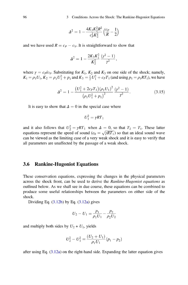
Δ
2
¼ 1 À
4K 3 K
2
1 R
2
c 2
P K
2
2
c P
R
À
1
2
and we have used R ¼ c P À c V . It is straightforward to show that
Δ
2
¼ 1 À
2K 3 K
2
1
K
2
2
γ
2
À 1
ð
Þ
γ 2 ,
where γ ¼ c P /c V . Substituting for K 1 , K 2 and K 3 on one side of the shock; namely,
K 1 ¼ ρ 1 U 1 , K 2 ¼ ρ 1 U
2
1 þ p 1 and K 3 ¼
1
2 U
2
1 þ c P T 1 (and using p 1 ¼ ρ 1 RT 1 ), we have
Δ
2
¼ 1 À
U
2
1 þ 2c P T 1
À
Á ρ 1 U 1
ð
Þ
2
ρ 1 U
2
1 þ p 1
À
Á 2
γ
2
À 1
ð
Þ
γ 2 :
ð3:15Þ
It is easy to show that Δ ¼ 0 in the special case where
U
2
1 ¼ γRT 1
and it also follows that U
2
2 ¼ γRT 1 when Δ ¼ 0, so that T 2 ¼ T 1 . These latter
equations represent the speed of sound (c 0 ¼
ffiffiffiffiffiffiffiffiffiffi ffi
γRT 1
p
) so that an ideal sound wave
can be viewed as the limiting case of a very weak shock and it is easy to verify that
all parameters are unaffected by the passage of a weak shock.
3.6 Rankine-Hugoniot Equations
These conservation equations, expressing the changes in the physical parameters
across the shock front, can be used to derive the Rankine-Hugoniot equations as
outlined below. As we shall see in due course, these equations can be combined to
produce some useful relationships between the parameters on either side of the
shock.
Dividing Eq. (3.12b) by Eq. (3.12a) gives
U 2 À U 1 ¼
p 1
ρ 1 U 1
À
p 2
ρ 2 U 2
and multiply both sides by U 2 + U 1 , yields
U
2
2 À U
2
1 ¼
U 2 þ U 1
ð
Þ
ρ 1 U 1
p 1 À p 2
ð
Þ
after using Eq. (3.12a) on the right-hand side. Expanding the latter equation gives
96
3 Conditions Across the Shock: The Rankine-Hugoniot Equations
2
¼ 1 À
4K 3 K
2
1 R
2
c 2
P K
2
2
c P
R
À
1
2
and we have used R ¼ c P À c V . It is straightforward to show that
Δ
2
¼ 1 À
2K 3 K
2
1
K
2
2
γ
2
À 1
ð
Þ
γ 2 ,
where γ ¼ c P /c V . Substituting for K 1 , K 2 and K 3 on one side of the shock; namely,
K 1 ¼ ρ 1 U 1 , K 2 ¼ ρ 1 U
2
1 þ p 1 and K 3 ¼
1
2 U
2
1 þ c P T 1 (and using p 1 ¼ ρ 1 RT 1 ), we have
Δ
2
¼ 1 À
U
2
1 þ 2c P T 1
À
Á ρ 1 U 1
ð
Þ
2
ρ 1 U
2
1 þ p 1
À
Á 2
γ
2
À 1
ð
Þ
γ 2 :
ð3:15Þ
It is easy to show that Δ ¼ 0 in the special case where
U
2
1 ¼ γRT 1
and it also follows that U
2
2 ¼ γRT 1 when Δ ¼ 0, so that T 2 ¼ T 1 . These latter
equations represent the speed of sound (c 0 ¼
ffiffiffiffiffiffiffiffiffiffi ffi
γRT 1
p
) so that an ideal sound wave
can be viewed as the limiting case of a very weak shock and it is easy to verify that
all parameters are unaffected by the passage of a weak shock.
3.6 Rankine-Hugoniot Equations
These conservation equations, expressing the changes in the physical parameters
across the shock front, can be used to derive the Rankine-Hugoniot equations as
outlined below. As we shall see in due course, these equations can be combined to
produce some useful relationships between the parameters on either side of the
shock.
Dividing Eq. (3.12b) by Eq. (3.12a) gives
U 2 À U 1 ¼
p 1
ρ 1 U 1
À
p 2
ρ 2 U 2
and multiply both sides by U 2 + U 1 , yields
U
2
2 À U
2
1 ¼
U 2 þ U 1
ð
Þ
ρ 1 U 1
p 1 À p 2
ð
Þ
after using Eq. (3.12a) on the right-hand side. Expanding the latter equation gives
96
3 Conditions Across the Shock: The Rankine-Hugoniot Equations