

General Relativity and Cosmology
401
and r 0 = R sin (a/R) is bounded by the value R. This is an elementary example of
a finite universe.
11.3 SCHWARZSCHILD METRIC
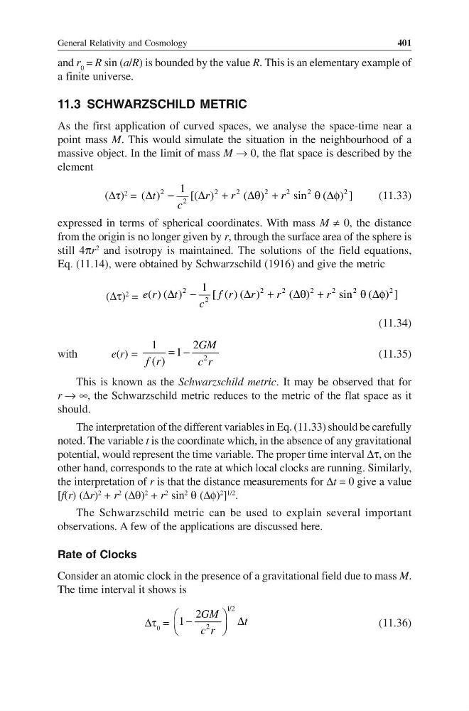
As the first application of curved spaces, we analyse the space-time near a
point mass M. This would simulate the situation in the neighbourhood of a
massive object. In the limit of mass M → 0, the flat space is described by the
element
(∆τ)
2
=
2
2
2
2
2
2
2
2
1
( )
[( )
( )
sin ( ) ]
t
r
r
r
c
∆ −
∆ +
∆θ +
θ ∆φ
(11.33)
expressed in terms of spherical coordinates. With mass M ≠ 0, the distance
from the origin is no longer given by r, through the surface area of the sphere is
still 4πr
2
and isotropy is maintained. The solutions of the field equations,
Eq. (11.14), were obtained by Schwarzschild (1916) and give the metric
(∆τ)
2
=
2
2
2
2
2
2
2
2
1
( ) ( )
[ ( ) ( )
( )
sin ( ) ]
e r
t
f r
r
r
r
c
∆ −
∆ +
∆θ +
θ ∆φ
(11.34)
with
e(r) =
2
1
2
1
( )
GM
f r
c r
= −
(11.35)
This is known as the Schwarzschild metric. It may be observed that for
r → ∞, the Schwarzschild metric reduces to the metric of the flat space as it
should.
The interpretation of the different variables in Eq. (11.33) should be carefully
noted. The variable t is the coordinate which, in the absence of any gravitational
potential, would represent the time variable. The proper time interval ∆τ, on the
other hand, corresponds to the rate at which local clocks are running. Similarly,
the interpretation of r is that the distance measurements for ∆t = 0 give a value
[f(r) (∆r)
2
+ r
2
(∆θ)
2
+ r
2
sin
2
θ (∆φ)
2
]
1/2
.
The Schwarzschild metric can be used to explain several important
observations. A few of the applications are discussed here.
Rate of Clocks
Consider an atomic clock in the presence of a gravitational field due to mass M.
The time interval it shows is
∆τ 0 =
1/2
2
2
1
GM
t
c r
−
∆
(11.36)
401
and r 0 = R sin (a/R) is bounded by the value R. This is an elementary example of
a finite universe.
11.3 SCHWARZSCHILD METRIC
As the first application of curved spaces, we analyse the space-time near a
point mass M. This would simulate the situation in the neighbourhood of a
massive object. In the limit of mass M → 0, the flat space is described by the
element
(∆τ)
2
=
2
2
2
2
2
2
2
2
1
( )
[( )
( )
sin ( ) ]
t
r
r
r
c
∆ −
∆ +
∆θ +
θ ∆φ
(11.33)
expressed in terms of spherical coordinates. With mass M ≠ 0, the distance
from the origin is no longer given by r, through the surface area of the sphere is
still 4πr
2
and isotropy is maintained. The solutions of the field equations,
Eq. (11.14), were obtained by Schwarzschild (1916) and give the metric
(∆τ)
2
=
2
2
2
2
2
2
2
2
1
( ) ( )
[ ( ) ( )
( )
sin ( ) ]
e r
t
f r
r
r
r
c
∆ −
∆ +
∆θ +
θ ∆φ
(11.34)
with
e(r) =
2
1
2
1
( )
GM
f r
c r
= −
(11.35)
This is known as the Schwarzschild metric. It may be observed that for
r → ∞, the Schwarzschild metric reduces to the metric of the flat space as it
should.
The interpretation of the different variables in Eq. (11.33) should be carefully
noted. The variable t is the coordinate which, in the absence of any gravitational
potential, would represent the time variable. The proper time interval ∆τ, on the
other hand, corresponds to the rate at which local clocks are running. Similarly,
the interpretation of r is that the distance measurements for ∆t = 0 give a value
[f(r) (∆r)
2
+ r
2
(∆θ)
2
+ r
2
sin
2
θ (∆φ)
2
]
1/2
.
The Schwarzschild metric can be used to explain several important
observations. A few of the applications are discussed here.
Rate of Clocks
Consider an atomic clock in the presence of a gravitational field due to mass M.
The time interval it shows is
∆τ 0 =
1/2
2
2
1
GM
t
c r
−
∆
(11.36)