

General Relativity and Cosmology
399
which follows from Eq. (11.12). For the special case of
0,
f
x
µ
∂ =
∂
Eq. (11.22)
simplifies to
f
dx
d
µ
∂
∂
τ
= constant.
(11.24)
These differential equations, i.e. Eq. (11.22) or Eq. (11.24), with Eq. (11.23),
determine the geodesics and hence the dynamics of a particle.
As an illustration, the metric tensor in Eq. (11.8) is considered for the case
of acceleration a in the x-direction,
g 00 =
2 2
11
01
10
2
2
2
1
1
,
,
a t
at
g
g
g
c
c
c
−
=−
=
=
(11.25)
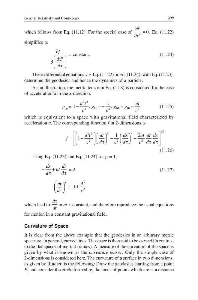
which is equivalent to a space with gravitational field characterized by
acceleration a. The corresponding function f in 2-dimensions is
f =
1/2
2
2
2 2
2
2
2
1
2
1
a t
dt
dx
at dt dx
d
d
d d
c
c
c
−
−
+
τ
τ
τ τ
(11.26)
Using Eq. (11.23) and Eq. (11.24) for µ = 1,
dx
dt
at
d
d
−
+
τ
τ
= A
(11.27)
2
dt
d
τ
=
2
2
1
A
c
+
which lead to
dx
dt
= at + constant, and therefore reproduce the usual equations
for motion in a constant gravitational field.
Curvature of Space
It is clear from the above example that the geodesics in an arbitrary metric
space are, in general, curved lines. The space is then said to be curved (in contrast
to the flat spaces of inertial frames). A measure of the curvature of the space is
given by what is known as the curvature tensor. Only the simple case of
2-dimensions is considered here. The curvature of a surface in two dimensions,
as given by Rindler, is the following: Draw the geodesics starting from a point
P, and consider the circle formed by the locus of points which are at a distance
399
which follows from Eq. (11.12). For the special case of
0,
f
x
µ
∂ =
∂
Eq. (11.22)
simplifies to
f
dx
d
µ
∂
∂
τ
= constant.
(11.24)
These differential equations, i.e. Eq. (11.22) or Eq. (11.24), with Eq. (11.23),
determine the geodesics and hence the dynamics of a particle.
As an illustration, the metric tensor in Eq. (11.8) is considered for the case
of acceleration a in the x-direction,
g 00 =
2 2
11
01
10
2
2
2
1
1
,
,
a t
at
g
g
g
c
c
c
−
=−
=
=
(11.25)
which is equivalent to a space with gravitational field characterized by
acceleration a. The corresponding function f in 2-dimensions is
f =
1/2
2
2
2 2
2
2
2
1
2
1
a t
dt
dx
at dt dx
d
d
d d
c
c
c
−
−
+
τ
τ
τ τ
(11.26)
Using Eq. (11.23) and Eq. (11.24) for µ = 1,
dx
dt
at
d
d
−
+
τ
τ
= A
(11.27)
2
dt
d
τ
=
2
2
1
A
c
+
which lead to
dx
dt
= at + constant, and therefore reproduce the usual equations
for motion in a constant gravitational field.
Curvature of Space
It is clear from the above example that the geodesics in an arbitrary metric
space are, in general, curved lines. The space is then said to be curved (in contrast
to the flat spaces of inertial frames). A measure of the curvature of the space is
given by what is known as the curvature tensor. Only the simple case of
2-dimensions is considered here. The curvature of a surface in two dimensions,
as given by Rindler, is the following: Draw the geodesics starting from a point
P, and consider the circle formed by the locus of points which are at a distance