

Elements of Modern Physics
180
equidistance is removed by the second term which, for these levels, has a value
of a
2
, 0, – a
2
/2, 0, – a
2
. The shifts in the transition frequencies are now given
by
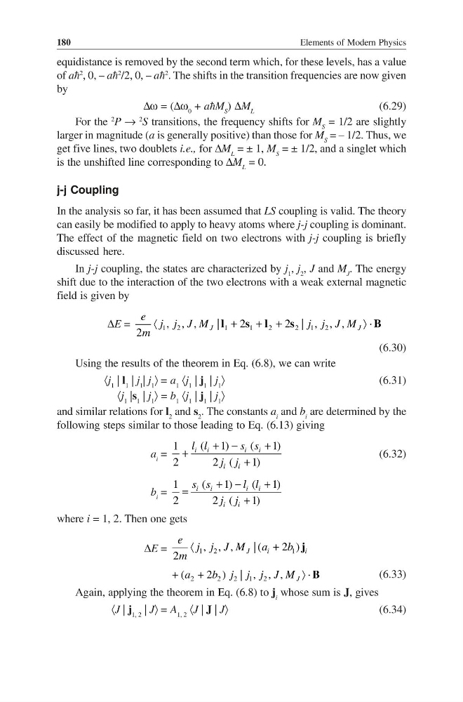
∆ω = (∆ω 0 + aM S ) ∆M L
(6.29)
For the
2
P →
2
S transitions, the frequency shifts for M S = 1/2 are slightly
larger in magnitude (a is generally positive) than those for M S = – 1/2. Thus, we
get five lines, two doublets i.e., for ∆M L = ± 1, M S = ± 1/2, and a singlet which
is the unshifted line corresponding to ∆M L = 0.
j-j Coupling
In the analysis so far, it has been assumed that LS coupling is valid. The theory
can easily be modified to apply to heavy atoms where j-j coupling is dominant.
The effect of the magnetic field on two electrons with j-j coupling is briefly
discussed here.
In j-j coupling, the states are characterized by j 1 , j 2 , J and M J . The energy
shift due to the interaction of the two electrons with a weak external magnetic
field is given by
∆E =
1
2
1
1
2
2
1
2
, , ,
|
2
2 | , , ,
2
J
J
e j j J M
j j J M
m
〈
+
+ +
〉 ⋅
l
s l
s
B
(6.30)
Using the results of the theorem in Eq. (6.8), we can write
〈j 1 | l 1 | j 1 | j 1 〉 = a 1 〈j 1 | j 1 | j 1 〉
(6.31)
〈j 1 |s 1 | j 1 〉 = b 1 〈j 1 | j 1 | j 1 〉
and similar relations for l 2 and s 2 . The constants a i and b i are determined by the
following steps similar to those leading to Eq. (6.13) giving
a i =
( 1)
(
1)
1
2
2 (
1 )
+ −
+
+
+
i i
i
i
i
i
l l
s s
j j
(6.32)
b i =
(
1)
( 1)
1
2
2 (
1 )
+ −
+
=
+
i
i
i i
i
i
s s
l l
j j
where i = 1, 2. Then one gets
∆E =
1
2
1
, , ,
| (
2 )
2
J
i
i
e j j J M a
b
m
〈
+
j
2
2
2
1
2
(
2 ) | , , , J
a
b j j j J M
+
+
〉 ⋅ B
(6.33)
Again, applying the theorem in Eq. (6.8) to j i whose sum is J, gives
〈J | j 1, 2 | J〉 = A 1, 2 〈J | J | J〉
(6.34)
180
equidistance is removed by the second term which, for these levels, has a value
of a
2
, 0, – a
2
/2, 0, – a
2
. The shifts in the transition frequencies are now given
by
∆ω = (∆ω 0 + aM S ) ∆M L
(6.29)
For the
2
P →
2
S transitions, the frequency shifts for M S = 1/2 are slightly
larger in magnitude (a is generally positive) than those for M S = – 1/2. Thus, we
get five lines, two doublets i.e., for ∆M L = ± 1, M S = ± 1/2, and a singlet which
is the unshifted line corresponding to ∆M L = 0.
j-j Coupling
In the analysis so far, it has been assumed that LS coupling is valid. The theory
can easily be modified to apply to heavy atoms where j-j coupling is dominant.
The effect of the magnetic field on two electrons with j-j coupling is briefly
discussed here.
In j-j coupling, the states are characterized by j 1 , j 2 , J and M J . The energy
shift due to the interaction of the two electrons with a weak external magnetic
field is given by
∆E =
1
2
1
1
2
2
1
2
, , ,
|
2
2 | , , ,
2
J
J
e j j J M
j j J M
m
〈
+
+ +
〉 ⋅
l
s l
s
B
(6.30)
Using the results of the theorem in Eq. (6.8), we can write
〈j 1 | l 1 | j 1 | j 1 〉 = a 1 〈j 1 | j 1 | j 1 〉
(6.31)
〈j 1 |s 1 | j 1 〉 = b 1 〈j 1 | j 1 | j 1 〉
and similar relations for l 2 and s 2 . The constants a i and b i are determined by the
following steps similar to those leading to Eq. (6.13) giving
a i =
( 1)
(
1)
1
2
2 (
1 )
+ −
+
+
+
i i
i
i
i
i
l l
s s
j j
(6.32)
b i =
(
1)
( 1)
1
2
2 (
1 )
+ −
+
=
+
i
i
i i
i
i
s s
l l
j j
where i = 1, 2. Then one gets
∆E =
1
2
1
, , ,
| (
2 )
2
J
i
i
e j j J M a
b
m
〈
+
j
2
2
2
1
2
(
2 ) | , , , J
a
b j j j J M
+
+
〉 ⋅ B
(6.33)
Again, applying the theorem in Eq. (6.8) to j i whose sum is J, gives
〈J | j 1, 2 | J〉 = A 1, 2 〈J | J | J〉
(6.34)