

Interaction with External Fields
179
Paschen-Back Effect
If the magnetic field is so strong that the splitting of the energy levels due to the
magnetic field is larger than the fine structure separation, is known as PaschenBack effect. In this case, H′ in Eq. (6.6) is treated as the main term and H 2
representing the spin-orbit interaction as a small perturbation, which makes the
calculations relatively simple.
In the absence of spin-orbit interaction, the unperturbed states may be
specified by the quantum numbers L, S, M L and M S . Taking the magnetic field
along the z-direction, the energy shift due to the magnetic field is given by
Eq. (6.6) as:
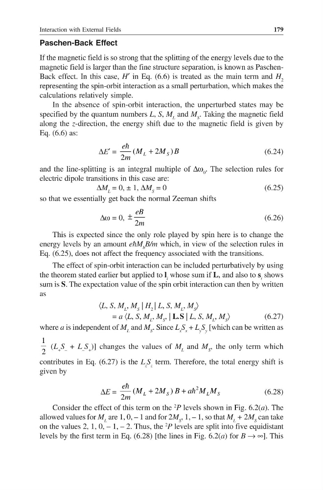
∆E′ =
(
2 )
2
L
S
e M
M B
m
+
(6.24)
and the line-splitting is an integral multiple of ∆ω 0 . The selection rules for
electric dipole transitions in this case are:
∆M L = 0, ± 1, ∆M S = 0
(6.25)
so that we essentially get back the normal Zeeman shifts
∆ω = 0, 2
±
eB
m
(6.26)
This is expected since the only role played by spin here is to change the
energy levels by an amount eM b B/m which, in view of the selection rules in
Eq. (6.25), does not affect the frequency associated with the transitions.
The effect of spin-orbit interaction can be included perturbatively by using
the theorem stated earlier but applied to l i whose sum if L, and also to s i shows
sum is S. The expectation value of the spin orbit interaction can then by written
as
〈L, S, M L , M S | H 2 | L, S, M L , M S 〉
= a 〈L, S, M L , M S , | L.S | L, S, M L , M S 〉
(6.27)
where a is independent of M L and M S . Since L x S x + L y S y [which can be written as
1
2
(L + S – + L – S + )] changes the values of M L and M S , the only term which
contributes in Eq. (6.27) is the L z S z term. Therefore, the total energy shift is
given by
∆E =
2
(
2 )
2
+
+
L
S
L
S
e M
M B a M M
m
(6.28)
Consider the effect of this term on the
2
P levels shown in Fig. 6.2(a). The
allowed values for M L are 1, 0, – 1 and for 2M S , 1, – 1, so that M L + 2M S can take
on the values 2, 1, 0, – 1, – 2. Thus, the
2
P levels are split into five equidistant
levels by the first term in Eq. (6.28) [the lines in Fig. 6.2(a) for B → ∞]. This
179
Paschen-Back Effect
If the magnetic field is so strong that the splitting of the energy levels due to the
magnetic field is larger than the fine structure separation, is known as PaschenBack effect. In this case, H′ in Eq. (6.6) is treated as the main term and H 2
representing the spin-orbit interaction as a small perturbation, which makes the
calculations relatively simple.
In the absence of spin-orbit interaction, the unperturbed states may be
specified by the quantum numbers L, S, M L and M S . Taking the magnetic field
along the z-direction, the energy shift due to the magnetic field is given by
Eq. (6.6) as:
∆E′ =
(
2 )
2
L
S
e M
M B
m
+
(6.24)
and the line-splitting is an integral multiple of ∆ω 0 . The selection rules for
electric dipole transitions in this case are:
∆M L = 0, ± 1, ∆M S = 0
(6.25)
so that we essentially get back the normal Zeeman shifts
∆ω = 0, 2
±
eB
m
(6.26)
This is expected since the only role played by spin here is to change the
energy levels by an amount eM b B/m which, in view of the selection rules in
Eq. (6.25), does not affect the frequency associated with the transitions.
The effect of spin-orbit interaction can be included perturbatively by using
the theorem stated earlier but applied to l i whose sum if L, and also to s i shows
sum is S. The expectation value of the spin orbit interaction can then by written
as
〈L, S, M L , M S | H 2 | L, S, M L , M S 〉
= a 〈L, S, M L , M S , | L.S | L, S, M L , M S 〉
(6.27)
where a is independent of M L and M S . Since L x S x + L y S y [which can be written as
1
2
(L + S – + L – S + )] changes the values of M L and M S , the only term which
contributes in Eq. (6.27) is the L z S z term. Therefore, the total energy shift is
given by
∆E =
2
(
2 )
2
+
+
L
S
L
S
e M
M B a M M
m
(6.28)
Consider the effect of this term on the
2
P levels shown in Fig. 6.2(a). The
allowed values for M L are 1, 0, – 1 and for 2M S , 1, – 1, so that M L + 2M S can take
on the values 2, 1, 0, – 1, – 2. Thus, the
2
P levels are split into five equidistant
levels by the first term in Eq. (6.28) [the lines in Fig. 6.2(a) for B → ∞]. This