

Elements of Modern Physics
176
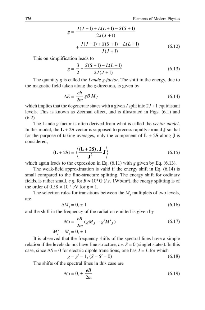
g =
(
1)
(
1)
(
1)
2 (
1)
+ +
+ −
+
+
J J
L L
S S
J J
(
1)
(
1)
(
1)
(
1)
+ +
+ −
+
+
+
J J
S S
L L
J J
(6.12)
This on simplification leads to
g =
3
( 1)
( 1)
2
2 (
1 )
+ −
+
+
+
S S
L L
J J
(6.13)
The quantity g is called the Lande g-factor. The shift in the energy, due to
the magnetic field taken along the z-direction, is given by
∆E = 2
J
eh gB M
m
(6.14)
which implies that the degenerate states with a given J split into 2J + 1 equidistant
levels. This is known as Zeeman effect, and is illustrated in Figs. (6.1) and
(6.2).
The Lande g-factor is often derived from what is called the vector model.
In this model, the L + 2S vector is supposed to precess rapidly around J so that
for the purpose of taking averages, only the component of L + 2S along J is
considered,
〈L + 2S〉 =
2
(
2 ).
+
L S J J
J
(6.15)
which again leads to the expression in Eq. (6.11) with g given by Eq. (6.13).
The weak-field approximation is valid if the energy shift in Eq. (6.14) is
small compared to the fine-structure splitting. The energy shift for ordinary
fields, is rather small, e.g. for B ≈ 10
4
G (i.e. 1Wb/m
2
), the energy splitting is of
the order of 0.58 × 10
–4
eV for g = 1.
The selection rules for transitions between the M J multiplets of two levels,
are:
∆M J = 0, ± 1
(6.16)
and the shift in the frequency of the radiation emitted is given by
∆ω =
(
)
2
− ′ ′
J
J
eB gM
g M
m
(6.17)
M J ′ – M J = 0, ± 1
It is observed that the frequency shifts of the spectral lines have a simple
relation if the levels do not have fine structure, i.e. S = 0 (singlet states). In this
case, since ∆S = 0 for electric dipole transitions, one has J = L for which
g = g′ = 1, (S = S′ = 0)
(6.18)
The shifts of the spectral lines in this case are
∆ω = 0, ± 2
eB
m
(6.19)
176
g =
(
1)
(
1)
(
1)
2 (
1)
+ +
+ −
+
+
J J
L L
S S
J J
(
1)
(
1)
(
1)
(
1)
+ +
+ −
+
+
+
J J
S S
L L
J J
(6.12)
This on simplification leads to
g =
3
( 1)
( 1)
2
2 (
1 )
+ −
+
+
+
S S
L L
J J
(6.13)
The quantity g is called the Lande g-factor. The shift in the energy, due to
the magnetic field taken along the z-direction, is given by
∆E = 2
J
eh gB M
m
(6.14)
which implies that the degenerate states with a given J split into 2J + 1 equidistant
levels. This is known as Zeeman effect, and is illustrated in Figs. (6.1) and
(6.2).
The Lande g-factor is often derived from what is called the vector model.
In this model, the L + 2S vector is supposed to precess rapidly around J so that
for the purpose of taking averages, only the component of L + 2S along J is
considered,
〈L + 2S〉 =
2
(
2 ).
+
L S J J
J
(6.15)
which again leads to the expression in Eq. (6.11) with g given by Eq. (6.13).
The weak-field approximation is valid if the energy shift in Eq. (6.14) is
small compared to the fine-structure splitting. The energy shift for ordinary
fields, is rather small, e.g. for B ≈ 10
4
G (i.e. 1Wb/m
2
), the energy splitting is of
the order of 0.58 × 10
–4
eV for g = 1.
The selection rules for transitions between the M J multiplets of two levels,
are:
∆M J = 0, ± 1
(6.16)
and the shift in the frequency of the radiation emitted is given by
∆ω =
(
)
2
− ′ ′
J
J
eB gM
g M
m
(6.17)
M J ′ – M J = 0, ± 1
It is observed that the frequency shifts of the spectral lines have a simple
relation if the levels do not have fine structure, i.e. S = 0 (singlet states). In this
case, since ∆S = 0 for electric dipole transitions, one has J = L for which
g = g′ = 1, (S = S′ = 0)
(6.18)
The shifts of the spectral lines in this case are
∆ω = 0, ± 2
eB
m
(6.19)