

Atoms and Molecules
149
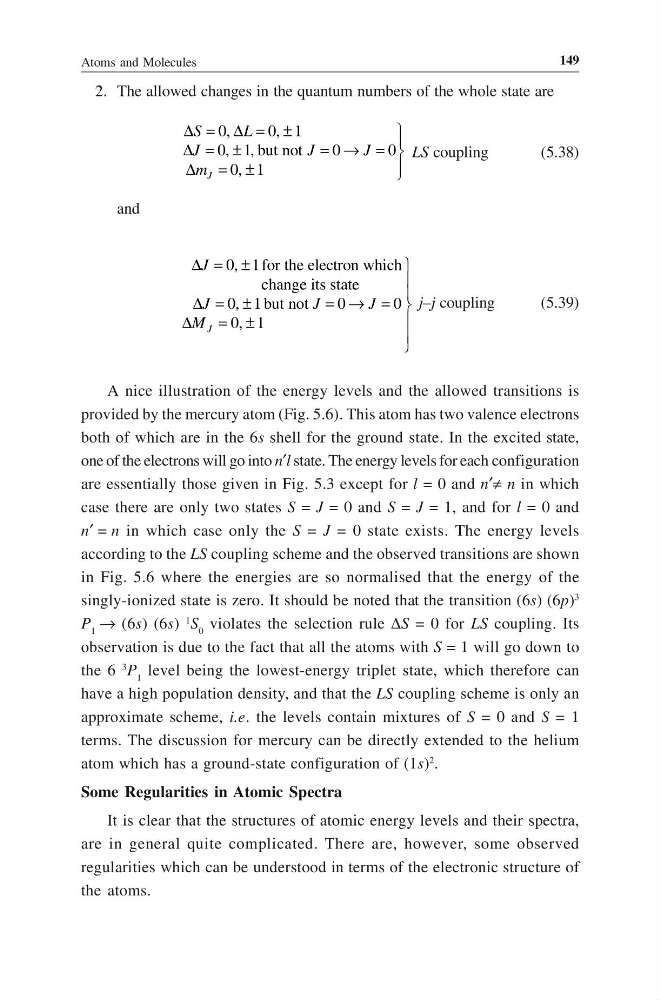
2. The allowed changes in the quantum numbers of the whole state are
0,
0, 1
0, 1, but not
0
0
0, 1
∆ = ∆ = ±
∆ = ±
= → =
∆ = ±
J
S
L
J
J
J
m
LS coupling
(5.38)
and
0, 1 for the electron which
change its state
0, 1 but not
0
0
0, 1
∆ = ±
∆ = ±
= → =
∆
= ±
J
J
J
J
J
M
j–j coupling
(5.39)
A nice illustration of the energy levels and the allowed transitions is
provided by the mercury atom (Fig. 5.6). This atom has two valence electrons
both of which are in the 6s shell for the ground state. In the excited state,
one of the electrons will go into n′l state. The energy levels for each configuration
are essentially those given in Fig. 5.3 except for l = 0 and n′≠ n in which
case there are only two states S = J = 0 and S = J = 1, and for l = 0 and
n′ = n in which case only the S = J = 0 state exists. The energy levels
according to the LS coupling scheme and the observed transitions are shown
in Fig. 5.6 where the energies are so normalised that the energy of the
singly-ionized state is zero. It should be noted that the transition (6s) (6p)
3
P 1 → (6s) (6s)
1
S 0 violates the selection rule ∆S = 0 for LS coupling. Its
observation is due to the fact that all the atoms with S = 1 will go down to
the 6
3
P 1 level being the lowest-energy triplet state, which therefore can
have a high population density, and that the LS coupling scheme is only an
approximate scheme, i.e. the levels contain mixtures of S = 0 and S = 1
terms. The discussion for mercury can be directly extended to the helium
atom which has a ground-state configuration of (1s)
2
.
Some Regularities in Atomic Spectra
It is clear that the structures of atomic energy levels and their spectra,
are in general quite complicated. There are, however, some observed
regularities which can be understood in terms of the electronic structure of
the atoms.
149
2. The allowed changes in the quantum numbers of the whole state are
0,
0, 1
0, 1, but not
0
0
0, 1
∆ = ∆ = ±
∆ = ±
= → =
∆ = ±
J
S
L
J
J
J
m
LS coupling
(5.38)
and
0, 1 for the electron which
change its state
0, 1 but not
0
0
0, 1
∆ = ±
∆ = ±
= → =
∆
= ±
J
J
J
J
J
M
j–j coupling
(5.39)
A nice illustration of the energy levels and the allowed transitions is
provided by the mercury atom (Fig. 5.6). This atom has two valence electrons
both of which are in the 6s shell for the ground state. In the excited state,
one of the electrons will go into n′l state. The energy levels for each configuration
are essentially those given in Fig. 5.3 except for l = 0 and n′≠ n in which
case there are only two states S = J = 0 and S = J = 1, and for l = 0 and
n′ = n in which case only the S = J = 0 state exists. The energy levels
according to the LS coupling scheme and the observed transitions are shown
in Fig. 5.6 where the energies are so normalised that the energy of the
singly-ionized state is zero. It should be noted that the transition (6s) (6p)
3
P 1 → (6s) (6s)
1
S 0 violates the selection rule ∆S = 0 for LS coupling. Its
observation is due to the fact that all the atoms with S = 1 will go down to
the 6
3
P 1 level being the lowest-energy triplet state, which therefore can
have a high population density, and that the LS coupling scheme is only an
approximate scheme, i.e. the levels contain mixtures of S = 0 and S = 1
terms. The discussion for mercury can be directly extended to the helium
atom which has a ground-state configuration of (1s)
2
.
Some Regularities in Atomic Spectra
It is clear that the structures of atomic energy levels and their spectra,
are in general quite complicated. There are, however, some observed
regularities which can be understood in terms of the electronic structure of
the atoms.