

Elements of Modern Physics
146
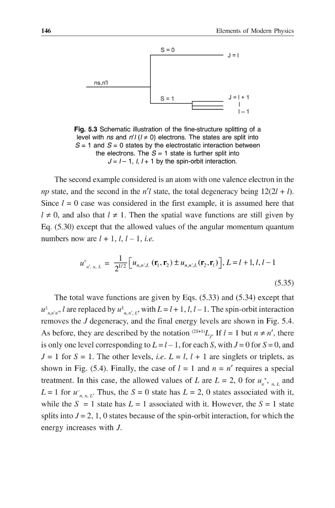
Fig. 5.3 Schematic illustration of the fine-structure splitting of a
level with ns and n′l (l ≠ 0) electrons. The states are split into
S = 1 and S = 0 states by the electrostatic interaction between
the electrons. The S = 1 state is further split into
J = l – 1, l, l + 1 by the spin-orbit interaction.
The second example considered is an atom with one valence electron in the
np state, and the second in the n′l state, the total degeneracy being 12(2l + l).
Since l = 0 case was considered in the first example, it is assumed here that
l ≠ 0, and also that l ≠ 1. Then the spatial wave functions are still given by
Eq. (5.30) except that the allowed values of the angular momentum quantum
numbers now are l + 1, l, l – 1, i.e.
u
±
n′, n, L
=
, ',
1 2
, ',
2 1
1/ 2
1
( , )
( , ) ,
1, , 1
2
±
= +
−
n n L
n n L
u
u
L l
ll
r r
r r
(5.35)
The total wave functions are given by Eqs. (5.33) and (5.34) except that
u
±
n,n’n′
, l are replaced by u
±
n, n′, L
, with L = l + 1, l, l – 1. The spin-orbit interaction
removes the J degeneracy, and the final energy levels are shown in Fig. 5.4.
As before, they are described by the notation
(2S+1)
L J . If l = 1 but n ≠ n′, there
is only one level corresponding to L = l – 1, for each S, with J = 0 for S = 0, and
J = 1 for S = 1. The other levels, i.e. L = l, l + 1 are singlets or triplets, as
shown in Fig. (5.4). Finally, the case of l = 1 and n = n′ requires a special
treatment. In this case, the allowed values of L are L = 2, 0 for u n
+
, n, L and
L = 1 for u
–
n, n, L
. Thus, the S = 0 state has L = 2, 0 states associated with it,
while the S = 1 state has L = 1 associated with it. However, the S = 1 state
splits into J = 2, 1, 0 states because of the spin-orbit interaction, for which the
energy increases with J.
146
Fig. 5.3 Schematic illustration of the fine-structure splitting of a
level with ns and n′l (l ≠ 0) electrons. The states are split into
S = 1 and S = 0 states by the electrostatic interaction between
the electrons. The S = 1 state is further split into
J = l – 1, l, l + 1 by the spin-orbit interaction.
The second example considered is an atom with one valence electron in the
np state, and the second in the n′l state, the total degeneracy being 12(2l + l).
Since l = 0 case was considered in the first example, it is assumed here that
l ≠ 0, and also that l ≠ 1. Then the spatial wave functions are still given by
Eq. (5.30) except that the allowed values of the angular momentum quantum
numbers now are l + 1, l, l – 1, i.e.
u
±
n′, n, L
=
, ',
1 2
, ',
2 1
1/ 2
1
( , )
( , ) ,
1, , 1
2
±
= +
−
n n L
n n L
u
u
L l
ll
r r
r r
(5.35)
The total wave functions are given by Eqs. (5.33) and (5.34) except that
u
±
n,n’n′
, l are replaced by u
±
n, n′, L
, with L = l + 1, l, l – 1. The spin-orbit interaction
removes the J degeneracy, and the final energy levels are shown in Fig. 5.4.
As before, they are described by the notation
(2S+1)
L J . If l = 1 but n ≠ n′, there
is only one level corresponding to L = l – 1, for each S, with J = 0 for S = 0, and
J = 1 for S = 1. The other levels, i.e. L = l, l + 1 are singlets or triplets, as
shown in Fig. (5.4). Finally, the case of l = 1 and n = n′ requires a special
treatment. In this case, the allowed values of L are L = 2, 0 for u n
+
, n, L and
L = 1 for u
–
n, n, L
. Thus, the S = 0 state has L = 2, 0 states associated with it,
while the S = 1 state has L = 1 associated with it. However, the S = 1 state
splits into J = 2, 1, 0 states because of the spin-orbit interaction, for which the
energy increases with J.