

3D Nanomagnetic Logic
271
the anisotropy constant for device and circuit simulation. However, this method has
several shortcomings:
• In easy-axis hysteresis loops, defects in a film act as strong nucleation centers and
the ‘true’ switching field cannot be attributed to the LLG-simulated values using
K u as ‘fitting’ parameter.
• The area of measurement is several 100 µm
2 whereas simulation area is a few µm
2
maximum.
• The time-scale of the experiment (several seconds in Hall-measurements) is not
related to the ‘virtual time-scales’ in the simulation, where the LLG is solved by
minimizing the energy term.
• The experiment is taken at room temperature, the simulations are at zero Kelvin,
hence thermally distributed switching fields are not covered.
Soon after, it became clear in NML research that only a focused spot of ion radiation
would solve both the non-reciprocity and effective field-coupling for a logic gate [23].
Further experiments showed, that different ion dose in a concentrated spot—called
Artificial Nucleation Center (ANC) from now on—were significantly changing the
switching field [25] . Franken et al. at the same time modeled and measured the
behavior of a step-like anisotropy change generated by FIB patterning of Co/Pt
strips [24] further confirming the findings of [25]. At this point it became obvious,
that detailed ANC modeling would be necessary to map the distributions found in
the experiment, and get reasonably low switching fields without using K u as simple
fitting parameter in the micromagnetic models.
3.2 ANC Modeling and Switching Field Distributions
Arrhenius-Type Models
In principle, the mean switching field of a nanomagnet can be described by the
so-called Sharrock-formalism [40]. It basically says, that the mean switching field
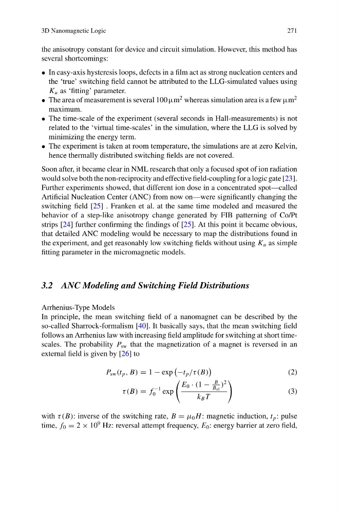
follows an Arrhenius law with increasing field amplitude for switching at short timescales. The probability P sw that the magnetization of a magnet is reversed in an
external field is given by [26] to
P sw (t p , B) = 1 − exp
−t p /τ (B)
(2)
τ (B) = f
−1
0 exp
E 0 · (1 −
B
B s0
)
2
k B T
(3)
with τ (B): inverse of the switching rate, B = μ 0 H : magnetic induction, t p : pulse
time, f 0 = 2 × 10
9 Hz: reversal attempt frequency, E 0 : energy barrier at zero field,
271
the anisotropy constant for device and circuit simulation. However, this method has
several shortcomings:
• In easy-axis hysteresis loops, defects in a film act as strong nucleation centers and
the ‘true’ switching field cannot be attributed to the LLG-simulated values using
K u as ‘fitting’ parameter.
• The area of measurement is several 100 µm
2 whereas simulation area is a few µm
2
maximum.
• The time-scale of the experiment (several seconds in Hall-measurements) is not
related to the ‘virtual time-scales’ in the simulation, where the LLG is solved by
minimizing the energy term.
• The experiment is taken at room temperature, the simulations are at zero Kelvin,
hence thermally distributed switching fields are not covered.
Soon after, it became clear in NML research that only a focused spot of ion radiation
would solve both the non-reciprocity and effective field-coupling for a logic gate [23].
Further experiments showed, that different ion dose in a concentrated spot—called
Artificial Nucleation Center (ANC) from now on—were significantly changing the
switching field [25] . Franken et al. at the same time modeled and measured the
behavior of a step-like anisotropy change generated by FIB patterning of Co/Pt
strips [24] further confirming the findings of [25]. At this point it became obvious,
that detailed ANC modeling would be necessary to map the distributions found in
the experiment, and get reasonably low switching fields without using K u as simple
fitting parameter in the micromagnetic models.
3.2 ANC Modeling and Switching Field Distributions
Arrhenius-Type Models
In principle, the mean switching field of a nanomagnet can be described by the
so-called Sharrock-formalism [40]. It basically says, that the mean switching field
follows an Arrhenius law with increasing field amplitude for switching at short timescales. The probability P sw that the magnetization of a magnet is reversed in an
external field is given by [26] to
P sw (t p , B) = 1 − exp
−t p /τ (B)
(2)
τ (B) = f
−1
0 exp
E 0 · (1 −
B
B s0
)
2
k B T
(3)
with τ (B): inverse of the switching rate, B = μ 0 H : magnetic induction, t p : pulse
time, f 0 = 2 × 10
9 Hz: reversal attempt frequency, E 0 : energy barrier at zero field,