

Electric-Field-Controlled MRAM: Physics and Applications
157
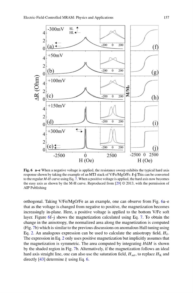
Fig. 6 a–e When a negative voltage is applied, the resistance sweep exhibits the typical hard axis
response shown by taking the example of an MTJ stack of V/Fe/MgO/Fe. f–j This can be converted
to the regular M-H curve using Eq. 7. When a positive voltage is applied, the hard axis now becomes
the easy axis as shown by the M-H curve. Reproduced from [29] © 2013, with the permission of
AIP Publishing
orthogonal. Taking V/Fe/MgO/Fe as an example, one can observe from Fig. 6a–e
that as the voltage is changed from negative to positive, the magnetization becomes
increasingly in-plane. Here, a positive voltage is applied to the bottom V/Fe soft
layer. Figure 6f–j shows the magnetization calculated using Eq. 7. To obtain the
change in the anisotropy, the normalized area along the magnetization is computed
(Fig. 7b) which is similar to the previous discussions on anomalous Hall tuning using
Eq. 2. An analogous expression can be used to calculate the anisotropy field, H k .
The expression in Eq. 2 only uses positive magnetization but implicitly assumes that
the magnetization is symmetric. The area computed by integrating HdM is shown
by the shaded region in Fig. 7b. Alternatively, if the magnetization follows an ideal
hard axis straight line, one can also use the saturation field, H sat , to replace H K and
directly [43] determine ξ using Eq. 6.
157
Fig. 6 a–e When a negative voltage is applied, the resistance sweep exhibits the typical hard axis
response shown by taking the example of an MTJ stack of V/Fe/MgO/Fe. f–j This can be converted
to the regular M-H curve using Eq. 7. When a positive voltage is applied, the hard axis now becomes
the easy axis as shown by the M-H curve. Reproduced from [29] © 2013, with the permission of
AIP Publishing
orthogonal. Taking V/Fe/MgO/Fe as an example, one can observe from Fig. 6a–e
that as the voltage is changed from negative to positive, the magnetization becomes
increasingly in-plane. Here, a positive voltage is applied to the bottom V/Fe soft
layer. Figure 6f–j shows the magnetization calculated using Eq. 7. To obtain the
change in the anisotropy, the normalized area along the magnetization is computed
(Fig. 7b) which is similar to the previous discussions on anomalous Hall tuning using
Eq. 2. An analogous expression can be used to calculate the anisotropy field, H k .
The expression in Eq. 2 only uses positive magnetization but implicitly assumes that
the magnetization is symmetric. The area computed by integrating HdM is shown
by the shaded region in Fig. 7b. Alternatively, if the magnetization follows an ideal
hard axis straight line, one can also use the saturation field, H sat , to replace H K and
directly [43] determine ξ using Eq. 6.