

156
J. Lourembam and J. Huang
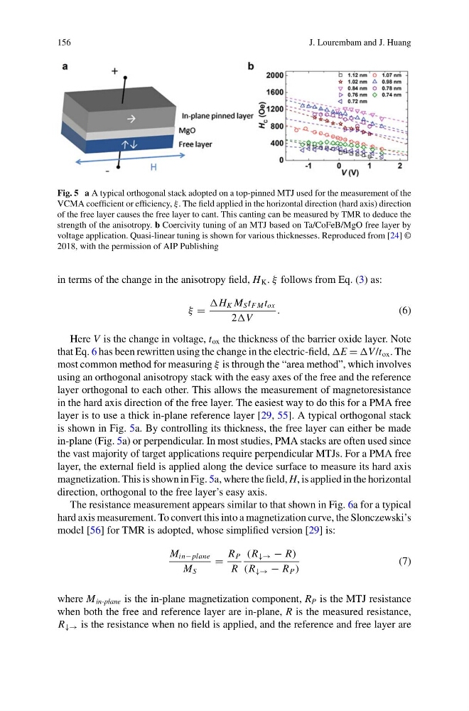
Fig. 5 a A typical orthogonal stack adopted on a top-pinned MTJ used for the measurement of the
VCMA coefficient or efficiency, ξ. The field applied in the horizontal direction (hard axis) direction
of the free layer causes the free layer to cant. This canting can be measured by TMR to deduce the
strength of the anisotropy. b Coercivity tuning of an MTJ based on Ta/CoFeB/MgO free layer by
voltage application. Quasi-linear tuning is shown for various thicknesses. Reproduced from [24] ©
2018, with the permission of AIP Publishing
in terms of the change in the anisotropy field, H K . ξ follows from Eq. (3) as:
ξ =
H K M S t F M t ox
2V
.
(6)
Here V is the change in voltage, t ox the thickness of the barrier oxide layer. Note
that Eq. 6 has been rewritten using the change in the electric-field, E = V /t ox . The
most common method for measuring ξ is through the “area method”, which involves
using an orthogonal anisotropy stack with the easy axes of the free and the reference
layer orthogonal to each other. This allows the measurement of magnetoresistance
in the hard axis direction of the free layer. The easiest way to do this for a PMA free
layer is to use a thick in-plane reference layer [29, 55]. A typical orthogonal stack
is shown in Fig. 5a. By controlling its thickness, the free layer can either be made
in-plane (Fig. 5a) or perpendicular. In most studies, PMA stacks are often used since
the vast majority of target applications require perpendicular MTJs. For a PMA free
layer, the external field is applied along the device surface to measure its hard axis
magnetization. This is shown in Fig. 5a, where the field, H, is applied in the horizontal
direction, orthogonal to the free layer’s easy axis.
The resistance measurement appears similar to that shown in Fig. 6a for a typical
hard axis measurement. To convert this into a magnetization curve, the Slonczewski’s
model [56] for TMR is adopted, whose simplified version [29] is:
M in− plane
M S
=
R P
R
(R ↓→ − R)
(R ↓→ − R P )
(7)
where M in-plane is the in-plane magnetization component, R P is the MTJ resistance
when both the free and reference layer are in-plane, R is the measured resistance,
R ↓→ is the resistance when no field is applied, and the reference and free layer are
J. Lourembam and J. Huang
Fig. 5 a A typical orthogonal stack adopted on a top-pinned MTJ used for the measurement of the
VCMA coefficient or efficiency, ξ. The field applied in the horizontal direction (hard axis) direction
of the free layer causes the free layer to cant. This canting can be measured by TMR to deduce the
strength of the anisotropy. b Coercivity tuning of an MTJ based on Ta/CoFeB/MgO free layer by
voltage application. Quasi-linear tuning is shown for various thicknesses. Reproduced from [24] ©
2018, with the permission of AIP Publishing
in terms of the change in the anisotropy field, H K . ξ follows from Eq. (3) as:
ξ =
H K M S t F M t ox
2V
.
(6)
Here V is the change in voltage, t ox the thickness of the barrier oxide layer. Note
that Eq. 6 has been rewritten using the change in the electric-field, E = V /t ox . The
most common method for measuring ξ is through the “area method”, which involves
using an orthogonal anisotropy stack with the easy axes of the free and the reference
layer orthogonal to each other. This allows the measurement of magnetoresistance
in the hard axis direction of the free layer. The easiest way to do this for a PMA free
layer is to use a thick in-plane reference layer [29, 55]. A typical orthogonal stack
is shown in Fig. 5a. By controlling its thickness, the free layer can either be made
in-plane (Fig. 5a) or perpendicular. In most studies, PMA stacks are often used since
the vast majority of target applications require perpendicular MTJs. For a PMA free
layer, the external field is applied along the device surface to measure its hard axis
magnetization. This is shown in Fig. 5a, where the field, H, is applied in the horizontal
direction, orthogonal to the free layer’s easy axis.
The resistance measurement appears similar to that shown in Fig. 6a for a typical
hard axis measurement. To convert this into a magnetization curve, the Slonczewski’s
model [56] for TMR is adopted, whose simplified version [29] is:
M in− plane
M S
=
R P
R
(R ↓→ − R)
(R ↓→ − R P )
(7)
where M in-plane is the in-plane magnetization component, R P is the MTJ resistance
when both the free and reference layer are in-plane, R is the measured resistance,
R ↓→ is the resistance when no field is applied, and the reference and free layer are