

Electric-Field-Controlled MRAM: Physics and Applications
155
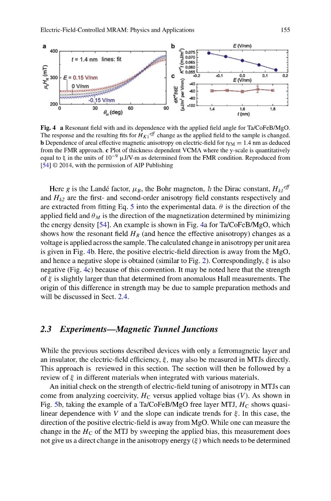
Fig. 4 a Resonant field with and its dependence with the applied field angle for Ta/CoFeB/MgO.
The response and the resulting fits for H K1
eff change as the applied field to the sample is changed.
b Dependence of areal effective magnetic anisotropy on electric-field for t FM = 1.4 nm as deduced
from the FMR approach. c Plot of thickness dependent VCMA where the y-scale is quantitatively
equal to ξ in the units of 10 −9 μJ/V-m as determined from the FMR condition. Reproduced from
[54] © 2014, with the permission of AIP Publishing
Here g is the Landé factor, μ B , the Bohr magneton, è the Dirac constant, H k1
eff
and H k2 are the first- and second-order anisotropy field constants respectively and
are extracted from fitting Eq. 5 into the experimental data. θ is the direction of the
applied field and θ M is the direction of the magnetization determined by minimizing
the energy density [54]. An example is shown in Fig. 4a for Ta/CoFeB/MgO, which
shows how the resonant field H R (and hence the effective anisotropy) changes as a
voltage is applied across the sample. The calculated change in anisotropy per unit area
is given in Fig. 4b. Here, the positive electric-field direction is away from the MgO,
and hence a negative slope is obtained (similar to Fig. 2). Correspondingly, ξ is also
negative (Fig. 4c) because of this convention. It may be noted here that the strength
of ξ is slightly larger than that determined from anomalous Hall measurements. The
origin of this difference in strength may be due to sample preparation methods and
will be discussed in Sect. 2.4.
2.3 Experiments—Magnetic Tunnel Junctions
While the previous sections described devices with only a ferromagnetic layer and
an insulator, the electric-field efficiency, ξ , may also be measured in MTJs directly.
This approach is reviewed in this section. The section will then be followed by a
review of ξ in different materials when integrated with various materials.
An initial check on the strength of electric-field tuning of anisotropy in MTJs can
come from analyzing coercivity, H C versus applied voltage bias (V ). As shown in
Fig. 5b, taking the example of a Ta/CoFeB/MgO free layer MTJ, H C shows quasilinear dependence with V and the slope can indicate trends for ξ. In this case, the
direction of the positive electric-field is away from MgO. While one can measure the
change in the H C of the MTJ by sweeping the applied bias, this measurement does
not give us a direct change in the anisotropy energy (ξ ) which needs to be determined
155
Fig. 4 a Resonant field with and its dependence with the applied field angle for Ta/CoFeB/MgO.
The response and the resulting fits for H K1
eff change as the applied field to the sample is changed.
b Dependence of areal effective magnetic anisotropy on electric-field for t FM = 1.4 nm as deduced
from the FMR approach. c Plot of thickness dependent VCMA where the y-scale is quantitatively
equal to ξ in the units of 10 −9 μJ/V-m as determined from the FMR condition. Reproduced from
[54] © 2014, with the permission of AIP Publishing
Here g is the Landé factor, μ B , the Bohr magneton, è the Dirac constant, H k1
eff
and H k2 are the first- and second-order anisotropy field constants respectively and
are extracted from fitting Eq. 5 into the experimental data. θ is the direction of the
applied field and θ M is the direction of the magnetization determined by minimizing
the energy density [54]. An example is shown in Fig. 4a for Ta/CoFeB/MgO, which
shows how the resonant field H R (and hence the effective anisotropy) changes as a
voltage is applied across the sample. The calculated change in anisotropy per unit area
is given in Fig. 4b. Here, the positive electric-field direction is away from the MgO,
and hence a negative slope is obtained (similar to Fig. 2). Correspondingly, ξ is also
negative (Fig. 4c) because of this convention. It may be noted here that the strength
of ξ is slightly larger than that determined from anomalous Hall measurements. The
origin of this difference in strength may be due to sample preparation methods and
will be discussed in Sect. 2.4.
2.3 Experiments—Magnetic Tunnel Junctions
While the previous sections described devices with only a ferromagnetic layer and
an insulator, the electric-field efficiency, ξ , may also be measured in MTJs directly.
This approach is reviewed in this section. The section will then be followed by a
review of ξ in different materials when integrated with various materials.
An initial check on the strength of electric-field tuning of anisotropy in MTJs can
come from analyzing coercivity, H C versus applied voltage bias (V ). As shown in
Fig. 5b, taking the example of a Ta/CoFeB/MgO free layer MTJ, H C shows quasilinear dependence with V and the slope can indicate trends for ξ. In this case, the
direction of the positive electric-field is away from MgO. While one can measure the
change in the H C of the MTJ by sweeping the applied bias, this measurement does
not give us a direct change in the anisotropy energy (ξ ) which needs to be determined