

Current-Driven Domain Wall Dynamics in Magnetic …
131
H SL
L
=
θ S H j a
2μ 0 |e − |M s t
(
m x ) × ×
u y =
θ S H j a
2μ 0 |e − |M s t
ˆ
z
.
(18)
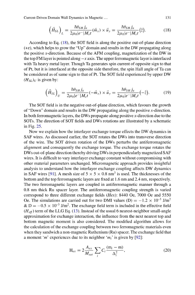
According to Eq. (18), the SOT field is along the positive out-of-plane direction
(+z), which helps to grow the “Up” domain and results in the DW propagating along
the positive x-direction. Because of the AFM coupling, magnetization of the DW in
the top FM layer is pointed along −x axis. The upper ferromagnetic layer is interfaced
with Ta heavy metal layer. Though Ta generates spin current of opposite sign to that
of Pt, but it is interfaced at the opposite side therefore, the spin Hall angle of Ta can
be considered as of same sign to that of Pt. The SOT field experienced by upper DW
(H SL ) U is given by:
H SL
U
=
θ S H j a
2μ 0 |e − |M s t
(− −
m x ) × ×
u y =
θ S H j a
2μ 0 |e − |M s t
−ˆ z
.
(19)
The SOT field is in the negative out-of-plane direction, which favours the growth
of “Down” domain and results in the DW propagating along the positive x-direction.
In both ferromagnetic layers, the DWs propagate along positive x-direction due to the
SOTs. The direction of SOT fields and DWs rotations are illustrated by a schematic
in Fig. 25.
Now we explain how the interlayer exchange torque effects the DW dynamics in
SAF wires. As discussed earlier, the SOT rotates the DWs into transverse direction
of the wire. The SOT driven rotation of the DWs perturbs the antiferromagnetic
alignment and consequently the exchange torque. The exchange torque rotates the
DWs out-of-plane direction thereby driving DWs in perpendicularly magnetized SAF
wires. It is difficult to vary interlayer exchange constant without compromising with
other material parameters unchanged. Micromagnetic approach provides insightful
analysis to understand how the interlayer exchange coupling affects DW dynamics
in SAF wires [91]. A mesh size of 5 × 5 × 0.8 nm
3 is used. The thicknesses of the
bottom and the top ferromagnetic layers are fixed at 1.6 nm and 2.4 nm, respectively.
The two ferromagnetic layers are coupled in antiferromagnetic manner through a
0.8 nm thick Ru spacer layer. The antiferromagnetic coupling strength is varied
correspond to three different exchange fields (Hex): 8440 Oe, 7000 Oe and 5550
Oe. The simulations are carried out for two DMI values (D) = −1.2 × 10
–3 J/m
2
& D = −0.5 × 10
–3 J/m
2 . The exchange field term is included in the effective field
(H eff ) term of the LLG Eq. (13). Instead of the usual 6 nearest-neighbor small-angle
approximation for exchange interaction, the influence from the next nearest top and
bottom magnetic moment is also considered. The modified algorithm allows for
the calculation of the exchange coupling between two ferromagnetic materials even
when they sandwich a non-magnetic Ruthenium (Ru) spacer. The exchange field that
a moment ‘m’ experiences due to its neighbor ‘m i ’ is given by [92]:
H ex = 2
A ex
M sat
i
C i
(m i − m)
2
i
,
(20)
131
H SL
L
=
θ S H j a
2μ 0 |e − |M s t
(
m x ) × ×
u y =
θ S H j a
2μ 0 |e − |M s t
ˆ
z
.
(18)
According to Eq. (18), the SOT field is along the positive out-of-plane direction
(+z), which helps to grow the “Up” domain and results in the DW propagating along
the positive x-direction. Because of the AFM coupling, magnetization of the DW in
the top FM layer is pointed along −x axis. The upper ferromagnetic layer is interfaced
with Ta heavy metal layer. Though Ta generates spin current of opposite sign to that
of Pt, but it is interfaced at the opposite side therefore, the spin Hall angle of Ta can
be considered as of same sign to that of Pt. The SOT field experienced by upper DW
(H SL ) U is given by:
H SL
U
=
θ S H j a
2μ 0 |e − |M s t
(− −
m x ) × ×
u y =
θ S H j a
2μ 0 |e − |M s t
−ˆ z
.
(19)
The SOT field is in the negative out-of-plane direction, which favours the growth
of “Down” domain and results in the DW propagating along the positive x-direction.
In both ferromagnetic layers, the DWs propagate along positive x-direction due to the
SOTs. The direction of SOT fields and DWs rotations are illustrated by a schematic
in Fig. 25.
Now we explain how the interlayer exchange torque effects the DW dynamics in
SAF wires. As discussed earlier, the SOT rotates the DWs into transverse direction
of the wire. The SOT driven rotation of the DWs perturbs the antiferromagnetic
alignment and consequently the exchange torque. The exchange torque rotates the
DWs out-of-plane direction thereby driving DWs in perpendicularly magnetized SAF
wires. It is difficult to vary interlayer exchange constant without compromising with
other material parameters unchanged. Micromagnetic approach provides insightful
analysis to understand how the interlayer exchange coupling affects DW dynamics
in SAF wires [91]. A mesh size of 5 × 5 × 0.8 nm
3 is used. The thicknesses of the
bottom and the top ferromagnetic layers are fixed at 1.6 nm and 2.4 nm, respectively.
The two ferromagnetic layers are coupled in antiferromagnetic manner through a
0.8 nm thick Ru spacer layer. The antiferromagnetic coupling strength is varied
correspond to three different exchange fields (Hex): 8440 Oe, 7000 Oe and 5550
Oe. The simulations are carried out for two DMI values (D) = −1.2 × 10
–3 J/m
2
& D = −0.5 × 10
–3 J/m
2 . The exchange field term is included in the effective field
(H eff ) term of the LLG Eq. (13). Instead of the usual 6 nearest-neighbor small-angle
approximation for exchange interaction, the influence from the next nearest top and
bottom magnetic moment is also considered. The modified algorithm allows for
the calculation of the exchange coupling between two ferromagnetic materials even
when they sandwich a non-magnetic Ruthenium (Ru) spacer. The exchange field that
a moment ‘m’ experiences due to its neighbor ‘m i ’ is given by [92]:
H ex = 2
A ex
M sat
i
C i
(m i − m)
2
i
,
(20)