

2.3 Mathematical Tools
51
whereas
(t; ω) and
(t; ω) are the real and imaginary parts of the complex strain
signal. Accordingly the rate of the harmonically oscillating strain signal has complex
representation
˙
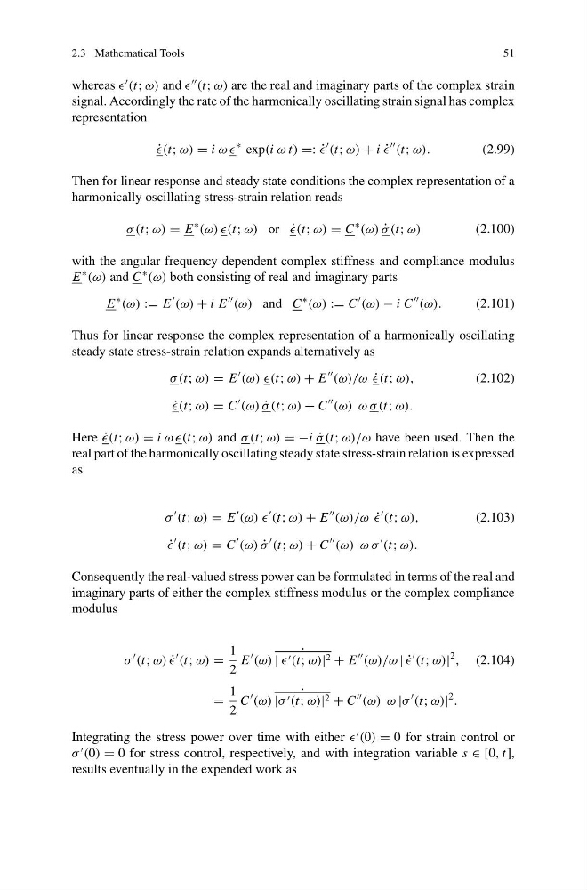
(t; ω) = i ω ω
∗ exp(i ω t) =: ˙
(t; ω) + i ˙
(t; ω).
(2.99)
Then for linear response and steady state conditions the complex representation of a
harmonically oscillating stress-strain relation reads
σ (t; ω) = E
∗
(ω) )(t; ω) or ˙
(t; ω) = C
∗
(ω) ˙
σ (t; ω)
(2.100)
with the angular frequency dependent complex stiffness and compliance modulus
E
∗
(ω) and C
∗
(ω) both consisting of real and imaginary parts
E
∗
(ω) := E
(ω) + i E
(ω) and C
∗
(ω) := C
(ω) − i C
(ω).
(2.101)
Thus for linear response the complex representation of a harmonically oscillating
steady state stress-strain relation expands alternatively as
σ (t; ω) = E
(ω) )(t; ω) + E
(ω)/ω ˙
(t; ω),
(2.102)
˙
(t; ω) = C
(ω) ˙
σ (t; ω) + C
(ω) ω σ (t; ω).
Here ˙
(t; ω) = i ω ω(t; ω) and σ (t; ω) = −i ˙
σ (t; ω)/ω have been used. Then the
real part of the harmonically oscillating steady state stress-strain relation is expressed
as
σ
(t; ω) = E
(ω) )
(t; ω) + E
(ω)/ω ˙
(t; ω),
(2.103)
˙
(t; ω) = C
(ω) ˙
σ
(t; ω) + C
(ω) ω σ
(t; ω).
Consequently the real-valued stress power can be formulated in terms of the real and
imaginary parts of either the complex stiffness modulus or the complex compliance
modulus
σ
(t; ω) ˙
(t; ω) =
1
2
E
(ω)
˙
| (t; ω)| 2 + E
(ω)/ω | ˙
(t; ω)|
2
, (2.104)
=
1
2
C
(ω)
˙
|σ (t; ω)| 2 + C
(ω) ω |σ
(t; ω)|
2
.
Integrating the stress power over time with either
(0) = 0 for strain control or
σ
(0) = 0 for stress control, respectively, and with integration variable s ∈ [0, t],
results eventually in the expended work as
51
whereas
(t; ω) and
(t; ω) are the real and imaginary parts of the complex strain
signal. Accordingly the rate of the harmonically oscillating strain signal has complex
representation
˙
(t; ω) = i ω ω
∗ exp(i ω t) =: ˙
(t; ω) + i ˙
(t; ω).
(2.99)
Then for linear response and steady state conditions the complex representation of a
harmonically oscillating stress-strain relation reads
σ (t; ω) = E
∗
(ω) )(t; ω) or ˙
(t; ω) = C
∗
(ω) ˙
σ (t; ω)
(2.100)
with the angular frequency dependent complex stiffness and compliance modulus
E
∗
(ω) and C
∗
(ω) both consisting of real and imaginary parts
E
∗
(ω) := E
(ω) + i E
(ω) and C
∗
(ω) := C
(ω) − i C
(ω).
(2.101)
Thus for linear response the complex representation of a harmonically oscillating
steady state stress-strain relation expands alternatively as
σ (t; ω) = E
(ω) )(t; ω) + E
(ω)/ω ˙
(t; ω),
(2.102)
˙
(t; ω) = C
(ω) ˙
σ (t; ω) + C
(ω) ω σ (t; ω).
Here ˙
(t; ω) = i ω ω(t; ω) and σ (t; ω) = −i ˙
σ (t; ω)/ω have been used. Then the
real part of the harmonically oscillating steady state stress-strain relation is expressed
as
σ
(t; ω) = E
(ω) )
(t; ω) + E
(ω)/ω ˙
(t; ω),
(2.103)
˙
(t; ω) = C
(ω) ˙
σ
(t; ω) + C
(ω) ω σ
(t; ω).
Consequently the real-valued stress power can be formulated in terms of the real and
imaginary parts of either the complex stiffness modulus or the complex compliance
modulus
σ
(t; ω) ˙
(t; ω) =
1
2
E
(ω)
˙
| (t; ω)| 2 + E
(ω)/ω | ˙
(t; ω)|
2
, (2.104)
=
1
2
C
(ω)
˙
|σ (t; ω)| 2 + C
(ω) ω |σ
(t; ω)|
2
.
Integrating the stress power over time with either
(0) = 0 for strain control or
σ
(0) = 0 for stress control, respectively, and with integration variable s ∈ [0, t],
results eventually in the expended work as