

38
2 Preliminaries
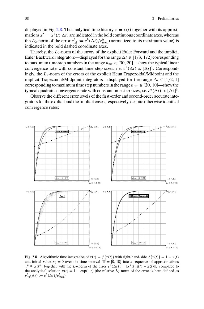
displayed in Fig. 2.8. The analytical time history x = x(t) together with its approximations x
h
= x
h
(t; are indicated in the bold continuous coordinate axes, whereas
the L 2 -norm of the error e
h
rel := e
h
((t)/e
h
max (normalized to its maximum value) is
indicated in the bold dashed coordinate axes.
Thereby, the L 2 -norm of the errors of the explicit Euler Forward and the implicit
Euler Backward integrators—displayed for the range ∈ [1/3, 1/2] corresponding
to maximum time step numbers in the range n mx ∈ [30, 20]—show the typical linear
convergence rate with constant time step sizes, i.e. e
h
((t) ∝ [
1 . Correspondingly, the L 2 -norm of the errors of the explicit Heun Trapezoidal/Midpoint and the
implicit Trapezoidal/Midpoint integrators—displayed for the range ∈ [1/2, 1]
corresponding to maximum time step numbers in the range n mx ∈ [20, 10]—show the
typical quadratic convergence rate with constant time step sizes, i.e. e
h
((t) ∝ [
2 .
Observe the different error levels of the first-order and second-order accurate integrators for the explicit and the implicit cases, respectively, despite otherwise identical
convergence rates:
t ∈ [0, 10]
x ∈ [0, 1]
Δt ∈ [0.¯ 3, 0.5]
e h
rel ∈ [0, 1]
Euler Forward
e h
max = 0.14946
Euler Forward
Euler Forward
Euler Forward
Euler Forward
Euler Forward
Euler Forward
Euler Forward
Euler Forward
Euler Forward
Euler Forward
t ∈ [0, 10]
x ∈ [0, 1]
Δt ∈ [0.¯ 3, 0.5]
e h
rel ∈ [0, 1]
Euler Backward
e h
max = 0.10990
Euler Backward
Euler Backward
Euler Backward
Euler Backward
Euler Backward
Euler Backward
Euler Backward
Euler Backward
Euler Backward
Euler Backward
t ∈ [0, 10]
x ∈ [0, 1]
Δt ∈ [0.5, 1.0]
e h
rel ∈ [0, 1]
Heun
e h
max = 0.19753
Heun Heun Heun Heun Heun Heun Heun Heun Heun Heun
t ∈ [0, 10]
x ∈ [0, 1]
Δt ∈ [0.5, 1.0]
e h
rel ∈ [0, 1]
Midpoint/Trapezoidal
e h
max = 0.04415
Midpoint/Trapezoidal
Midpoint/Trapezoidal
Midpoint/Trapezoidal
Midpoint/Trapezoidal
Midpoint/Trapezoidal
Midpoint/Trapezoidal
Midpoint/Trapezoidal
Midpoint/Trapezoidal
Midpoint/Trapezoidal
Midpoint/Trapezoidal
Fig. 2.8 Algorithmic time integration of ˙
x(t) = f
x(t)
with right-hand-side f
x(t)
= 1 − x(t)
and initial value x 0 = 0 over the time interval T = [0, 10] into a sequence of approximations
x n ≈ x(t n ) together with the L 2 -norm of the error e h ((t) := =x h (t; − x(t) 2 compared to
the analytical solution x(t) = 1 − exp(−t) (the relative L 2 -norm of the error is here defined as
e h
rel ((t) := e h ((t)/e h
max )
2 Preliminaries
displayed in Fig. 2.8. The analytical time history x = x(t) together with its approximations x
h
= x
h
(t; are indicated in the bold continuous coordinate axes, whereas
the L 2 -norm of the error e
h
rel := e
h
((t)/e
h
max (normalized to its maximum value) is
indicated in the bold dashed coordinate axes.
Thereby, the L 2 -norm of the errors of the explicit Euler Forward and the implicit
Euler Backward integrators—displayed for the range ∈ [1/3, 1/2] corresponding
to maximum time step numbers in the range n mx ∈ [30, 20]—show the typical linear
convergence rate with constant time step sizes, i.e. e
h
((t) ∝ [
1 . Correspondingly, the L 2 -norm of the errors of the explicit Heun Trapezoidal/Midpoint and the
implicit Trapezoidal/Midpoint integrators—displayed for the range ∈ [1/2, 1]
corresponding to maximum time step numbers in the range n mx ∈ [20, 10]—show the
typical quadratic convergence rate with constant time step sizes, i.e. e
h
((t) ∝ [
2 .
Observe the different error levels of the first-order and second-order accurate integrators for the explicit and the implicit cases, respectively, despite otherwise identical
convergence rates:
t ∈ [0, 10]
x ∈ [0, 1]
Δt ∈ [0.¯ 3, 0.5]
e h
rel ∈ [0, 1]
Euler Forward
e h
max = 0.14946
Euler Forward
Euler Forward
Euler Forward
Euler Forward
Euler Forward
Euler Forward
Euler Forward
Euler Forward
Euler Forward
Euler Forward
t ∈ [0, 10]
x ∈ [0, 1]
Δt ∈ [0.¯ 3, 0.5]
e h
rel ∈ [0, 1]
Euler Backward
e h
max = 0.10990
Euler Backward
Euler Backward
Euler Backward
Euler Backward
Euler Backward
Euler Backward
Euler Backward
Euler Backward
Euler Backward
Euler Backward
t ∈ [0, 10]
x ∈ [0, 1]
Δt ∈ [0.5, 1.0]
e h
rel ∈ [0, 1]
Heun
e h
max = 0.19753
Heun Heun Heun Heun Heun Heun Heun Heun Heun Heun
t ∈ [0, 10]
x ∈ [0, 1]
Δt ∈ [0.5, 1.0]
e h
rel ∈ [0, 1]
Midpoint/Trapezoidal
e h
max = 0.04415
Midpoint/Trapezoidal
Midpoint/Trapezoidal
Midpoint/Trapezoidal
Midpoint/Trapezoidal
Midpoint/Trapezoidal
Midpoint/Trapezoidal
Midpoint/Trapezoidal
Midpoint/Trapezoidal
Midpoint/Trapezoidal
Midpoint/Trapezoidal
Fig. 2.8 Algorithmic time integration of ˙
x(t) = f
x(t)
with right-hand-side f
x(t)
= 1 − x(t)
and initial value x 0 = 0 over the time interval T = [0, 10] into a sequence of approximations
x n ≈ x(t n ) together with the L 2 -norm of the error e h ((t) := =x h (t; − x(t) 2 compared to
the analytical solution x(t) = 1 − exp(−t) (the relative L 2 -norm of the error is here defined as
e h
rel ((t) := e h ((t)/e h
max )