

2.2 Computational Tools
37
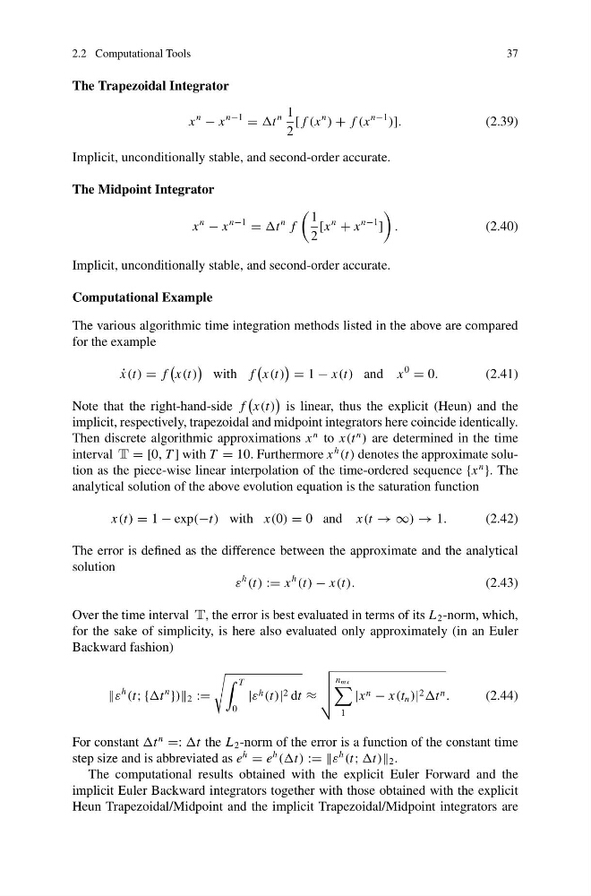
The Trapezoidal Integrator
x
n
− x
n−1
= t
n 1
2
[ f (x
n
) + f (x
n−1
)].
(2.39)
Implicit, unconditionally stable, and second-order accurate.
The Midpoint Integrator
x
n
− x
n−1
= t
n f
1
2
[x
n
+ x
n−1
]
.
(2.40)
Implicit, unconditionally stable, and second-order accurate.
Computational Example
The various algorithmic time integration methods listed in the above are compared
for the example
˙
x(t) = f
x(t)
with f
x(t)
= 1 − x(t) and x
0
= 0.
(2.41)
Note that the right-hand-side f
x(t)
is linear, thus the explicit (Heun) and the
implicit, respectively, trapezoidal and midpoint integrators here coincide identically.
Then discrete algorithmic approximations x
n to x(t
n
) are determined in the time
interval T = [0, T ] with T = 10. Furthermore x
h
(t) denotes the approximate solution as the piece-wise linear interpolation of the time-ordered sequence {x
n
}. The
analytical solution of the above evolution equation is the saturation function
x(t) = 1 − exp(−t) with x(0) = 0 and x(t → ∞) → 1.
(2.42)
The error is defined as the difference between the approximate and the analytical
solution
ε
h
(t) := x
h
(t) − x(t).
(2.43)
Over the time interval T, the error is best evaluated in terms of its L 2 -norm, which,
for the sake of simplicity, is here also evaluated only approximately (in an Euler
Backward fashion)
ε
h
(t; {t
n
}) 2 :=
T
0
|ε h (t)| 2 dt ≈
n mx
1
|x n − x(t n )| 2 t n .
(2.44)
For constant t
n
=: t the L 2 -norm of the error is a function of the constant time
step size and is abbreviated as e
h
= e
h
((t) := =ε
h
(t; t) 2 .
The computational results obtained with the explicit Euler Forward and the
implicit Euler Backward integrators together with those obtained with the explicit
Heun Trapezoidal/Midpoint and the implicit Trapezoidal/Midpoint integrators are
37
The Trapezoidal Integrator
x
n
− x
n−1
= t
n 1
2
[ f (x
n
) + f (x
n−1
)].
(2.39)
Implicit, unconditionally stable, and second-order accurate.
The Midpoint Integrator
x
n
− x
n−1
= t
n f
1
2
[x
n
+ x
n−1
]
.
(2.40)
Implicit, unconditionally stable, and second-order accurate.
Computational Example
The various algorithmic time integration methods listed in the above are compared
for the example
˙
x(t) = f
x(t)
with f
x(t)
= 1 − x(t) and x
0
= 0.
(2.41)
Note that the right-hand-side f
x(t)
is linear, thus the explicit (Heun) and the
implicit, respectively, trapezoidal and midpoint integrators here coincide identically.
Then discrete algorithmic approximations x
n to x(t
n
) are determined in the time
interval T = [0, T ] with T = 10. Furthermore x
h
(t) denotes the approximate solution as the piece-wise linear interpolation of the time-ordered sequence {x
n
}. The
analytical solution of the above evolution equation is the saturation function
x(t) = 1 − exp(−t) with x(0) = 0 and x(t → ∞) → 1.
(2.42)
The error is defined as the difference between the approximate and the analytical
solution
ε
h
(t) := x
h
(t) − x(t).
(2.43)
Over the time interval T, the error is best evaluated in terms of its L 2 -norm, which,
for the sake of simplicity, is here also evaluated only approximately (in an Euler
Backward fashion)
ε
h
(t; {t
n
}) 2 :=
T
0
|ε h (t)| 2 dt ≈
n mx
1
|x n − x(t n )| 2 t n .
(2.44)
For constant t
n
=: t the L 2 -norm of the error is a function of the constant time
step size and is abbreviated as e
h
= e
h
((t) := =ε
h
(t; t) 2 .
The computational results obtained with the explicit Euler Forward and the
implicit Euler Backward integrators together with those obtained with the explicit
Heun Trapezoidal/Midpoint and the implicit Trapezoidal/Midpoint integrators are