

2.2 Computational Tools
39
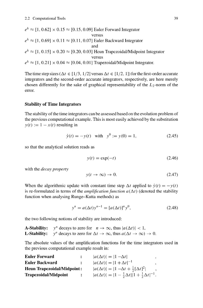
e
h
≈ [1, 0.62] × 0.15 ≈ [0.15, 0.09] Euler Forward Integrator
versus
e
h
≈ [1, 0.69] × 0.11 ≈ [0.11, 0.07] Euler Backward Integrator
and
e
h
≈ [1, 0.15] × 0.20 ≈ [0.20, 0.03] Heun Trapezoidal/Midpoint Integrator
versus
e
h
≈ [1, 0.21] × 0.04 ≈ [0.04, 0.01] Trapezoidal/Midpoint Integrator.
The time step sizes (t ∈ [1/3, 1/2] versus t ∈ [1/2, 1]) for the first-order accurate
integrators and the second-order accurate integrators, respectively, are here merely
chosen differently for the sake of graphical representability of the L 2 -norm of the
error.
Stability of Time Integrators
The stability of the time integrators can be assessed based on the evolution problem of
the previous computational example. This is most easily achieved by the substitution
y(t) := 1 − x(t) resulting in
˙
y(t) = −y(t) with y
0
:= y(0) = 1,
(2.45)
so that the analytical solution reads as
y(t) = exp(−t)
(2.46)
with the decay property
y(t → ∞) → 0.
(2.47)
When the algorithmic update with constant time step t applied to ˙
y(t) = −y(t)
is re-formulated in terms of the amplification function a((t) (denoted the stability
function when analysing Runge–Kutta methods) as
y
n
= a((t)y
n−1
= [a((t)]
n y
0
,
(2.48)
the two following notions of stability are introduced:
A-Stability: y
n decays to zero for n → ∞, thus |a((t)| < 1,
L-Stability: y
n decays to zero for t → ∞, thus a((t → ∞) → 0.
The absolute values of the amplification functions for the time integrators used in
the previous computational example result in:
Euler Forward
:
|a((t)| = |1 −t|
,
Euler Backward
:
|a((t)| = |1 +t|
−1
,
Heun Trapezoidal/Midpoint :
|a((t)| = |1 −t +
1
2
[t]
2
|
,
Trapezoidal/Midpoint
:
|a((t)| = |1 −
1
2
t||1 +
1
2
t|
−1
.
39
e
h
≈ [1, 0.62] × 0.15 ≈ [0.15, 0.09] Euler Forward Integrator
versus
e
h
≈ [1, 0.69] × 0.11 ≈ [0.11, 0.07] Euler Backward Integrator
and
e
h
≈ [1, 0.15] × 0.20 ≈ [0.20, 0.03] Heun Trapezoidal/Midpoint Integrator
versus
e
h
≈ [1, 0.21] × 0.04 ≈ [0.04, 0.01] Trapezoidal/Midpoint Integrator.
The time step sizes (t ∈ [1/3, 1/2] versus t ∈ [1/2, 1]) for the first-order accurate
integrators and the second-order accurate integrators, respectively, are here merely
chosen differently for the sake of graphical representability of the L 2 -norm of the
error.
Stability of Time Integrators
The stability of the time integrators can be assessed based on the evolution problem of
the previous computational example. This is most easily achieved by the substitution
y(t) := 1 − x(t) resulting in
˙
y(t) = −y(t) with y
0
:= y(0) = 1,
(2.45)
so that the analytical solution reads as
y(t) = exp(−t)
(2.46)
with the decay property
y(t → ∞) → 0.
(2.47)
When the algorithmic update with constant time step t applied to ˙
y(t) = −y(t)
is re-formulated in terms of the amplification function a((t) (denoted the stability
function when analysing Runge–Kutta methods) as
y
n
= a((t)y
n−1
= [a((t)]
n y
0
,
(2.48)
the two following notions of stability are introduced:
A-Stability: y
n decays to zero for n → ∞, thus |a((t)| < 1,
L-Stability: y
n decays to zero for t → ∞, thus a((t → ∞) → 0.
The absolute values of the amplification functions for the time integrators used in
the previous computational example result in:
Euler Forward
:
|a((t)| = |1 −t|
,
Euler Backward
:
|a((t)| = |1 +t|
−1
,
Heun Trapezoidal/Midpoint :
|a((t)| = |1 −t +
1
2
[t]
2
|
,
Trapezoidal/Midpoint
:
|a((t)| = |1 −
1
2
t||1 +
1
2
t|
−1
.