

5.1 St. Venant Model
201
σ p ⇐ σ p + E ˙
e = σ p + E [˙ − ˙
p ].
(5.31)
Note that once the kinematic constraint ˙
e = ˙
− ˙
p = 0 is satisfied, the total and the
plastic stress coincide σ = σ p .
5.1.2 Specific St. Venant Model: Algorithmic Update
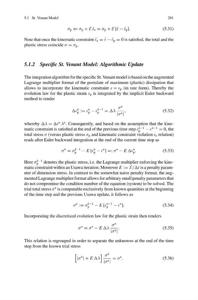
The integration algorithm for the specific St. Venant model is based on the augmented
Lagrange multiplier format of the postulate of maximum (plastic) dissipation that
allows to incorporate the kinematic constraint = p (in rate form). Thereby the
evolution law for the plastic strain p is integrated by the implicit Euler backward
method to render
n
p :=
n
p −
n−1
p
= λ
σ
n
|σ n |
,
(5.32)
whereby λ = t
n
λ
n . Consequently, and based on the assumption that the kinematic constraint is satisfied at the end of the previous time step
n−1
p
−
n−1
= 0, the
total stress σ (versus plastic stress σ p and kinematic constraint violation e relation)
reads after Euler backward integration at the end of the current time step as
σ
n
= σ
k−1
p
− E [
n
p −
n
] =: σ
− E
n
p .
(5.33)
Here σ
k−1
p
denotes the plastic stress, i.e. the Lagrange multiplier enforcing the kinematic constraint within an Usawa iteration. Moreover E := E//t is a penalty parameter of dimension stress. In contrast to the somewhat naive penalty format, the augmented Lagrange multiplier format allows for arbitrary small penalty parameters that
do not compromise the condition number of the equation (system) to be solved. The
trial total stress σ
is computable exclusively from known quantities at the beginning
of the time step and the previous Usawa update, it follows as
σ
:= σ
k−1
p
− E [
n−1
p
−
n
].
(5.34)
Incorporating the discretized evolution law for the plastic strain then renders
σ
n
= σ
− E λ
σ
n
|σ n |
.
(5.35)
This relation is regrouped in order to separate the unknowns at the end of the time
step from the known trial stress
|σ
n
| + E λ
σ
n
|σ n |
= σ
.
(5.36)
201
σ p ⇐ σ p + E ˙
e = σ p + E [˙ − ˙
p ].
(5.31)
Note that once the kinematic constraint ˙
e = ˙
− ˙
p = 0 is satisfied, the total and the
plastic stress coincide σ = σ p .
5.1.2 Specific St. Venant Model: Algorithmic Update
The integration algorithm for the specific St. Venant model is based on the augmented
Lagrange multiplier format of the postulate of maximum (plastic) dissipation that
allows to incorporate the kinematic constraint = p (in rate form). Thereby the
evolution law for the plastic strain p is integrated by the implicit Euler backward
method to render
n
p :=
n
p −
n−1
p
= λ
σ
n
|σ n |
,
(5.32)
whereby λ = t
n
λ
n . Consequently, and based on the assumption that the kinematic constraint is satisfied at the end of the previous time step
n−1
p
−
n−1
= 0, the
total stress σ (versus plastic stress σ p and kinematic constraint violation e relation)
reads after Euler backward integration at the end of the current time step as
σ
n
= σ
k−1
p
− E [
n
p −
n
] =: σ
− E
n
p .
(5.33)
Here σ
k−1
p
denotes the plastic stress, i.e. the Lagrange multiplier enforcing the kinematic constraint within an Usawa iteration. Moreover E := E//t is a penalty parameter of dimension stress. In contrast to the somewhat naive penalty format, the augmented Lagrange multiplier format allows for arbitrary small penalty parameters that
do not compromise the condition number of the equation (system) to be solved. The
trial total stress σ
is computable exclusively from known quantities at the beginning
of the time step and the previous Usawa update, it follows as
σ
:= σ
k−1
p
− E [
n−1
p
−
n
].
(5.34)
Incorporating the discretized evolution law for the plastic strain then renders
σ
n
= σ
− E λ
σ
n
|σ n |
.
(5.35)
This relation is regrouped in order to separate the unknowns at the end of the time
step from the known trial stress
|σ
n
| + E λ
σ
n
|σ n |
= σ
.
(5.36)