

202
5 Plasticity
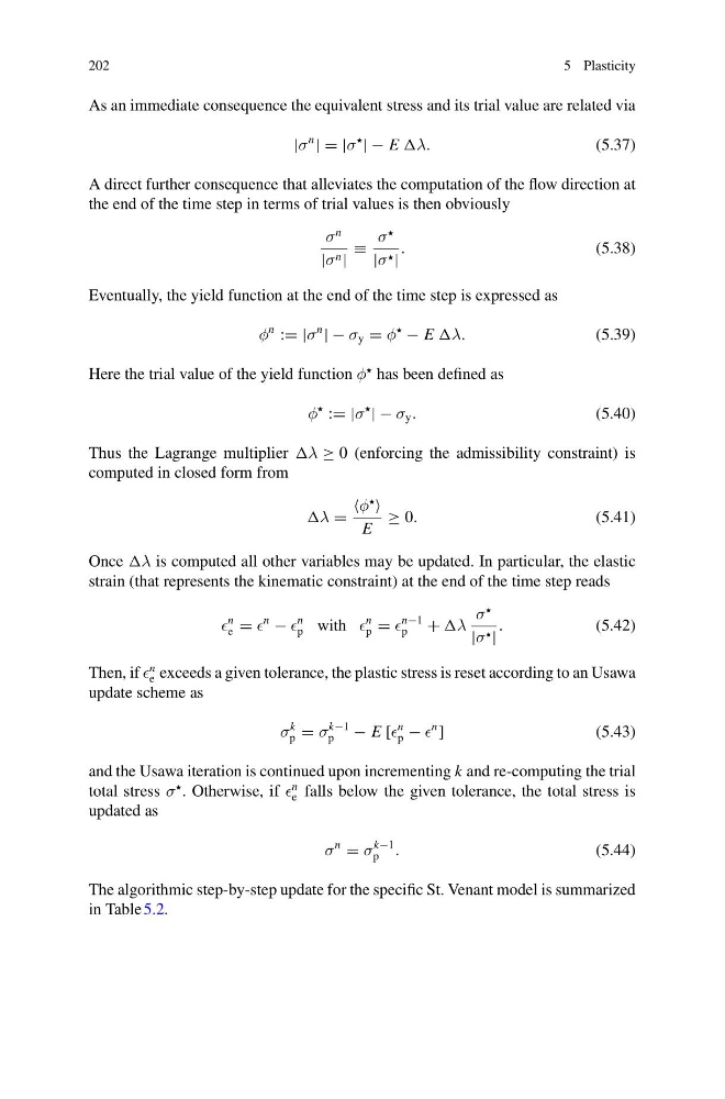
As an immediate consequence the equivalent stress and its trial value are related via
|σ
n
| = |σ
| − E λ.
(5.37)
A direct further consequence that alleviates the computation of the flow direction at
the end of the time step in terms of trial values is then obviously
σ
n
|σ n |
≡
σ
|σ |
.
(5.38)
Eventually, the yield function at the end of the time step is expressed as
φ
n
:= |σ
n
| − σ y = φ
− E λ.
(5.39)
Here the trial value of the yield function φ
has been defined as
φ
:= |σ
| − σ y .
(5.40)
Thus the Lagrange multiplier λ ≥ 0 (enforcing the admissibility constraint) is
computed in closed form from
λ =
φ
E
≥ 0.
(5.41)
Once λ is computed all other variables may be updated. In particular, the elastic
strain (that represents the kinematic constraint) at the end of the time step reads
n
e =
n
−
n
p with
n
p =
n−1
p
+ λ
σ
|σ |
.
(5.42)
Then, if
n
e exceeds a given tolerance, the plastic stress is reset according to an Usawa
update scheme as
σ
k
p = σ
k−1
p
− E [
n
p −
n
]
(5.43)
and the Usawa iteration is continued upon incrementing k and re-computing the trial
total stress σ
. Otherwise, if
n
e falls below the given tolerance, the total stress is
updated as
σ
n
= σ
k−1
p .
(5.44)
The algorithmic step-by-step update for the specific St. Venant model is summarized
in Table 5.2.
5 Plasticity
As an immediate consequence the equivalent stress and its trial value are related via
|σ
n
| = |σ
| − E λ.
(5.37)
A direct further consequence that alleviates the computation of the flow direction at
the end of the time step in terms of trial values is then obviously
σ
n
|σ n |
≡
σ
|σ |
.
(5.38)
Eventually, the yield function at the end of the time step is expressed as
φ
n
:= |σ
n
| − σ y = φ
− E λ.
(5.39)
Here the trial value of the yield function φ
has been defined as
φ
:= |σ
| − σ y .
(5.40)
Thus the Lagrange multiplier λ ≥ 0 (enforcing the admissibility constraint) is
computed in closed form from
λ =
φ
E
≥ 0.
(5.41)
Once λ is computed all other variables may be updated. In particular, the elastic
strain (that represents the kinematic constraint) at the end of the time step reads
n
e =
n
−
n
p with
n
p =
n−1
p
+ λ
σ
|σ |
.
(5.42)
Then, if
n
e exceeds a given tolerance, the plastic stress is reset according to an Usawa
update scheme as
σ
k
p = σ
k−1
p
− E [
n
p −
n
]
(5.43)
and the Usawa iteration is continued upon incrementing k and re-computing the trial
total stress σ
. Otherwise, if
n
e falls below the given tolerance, the total stress is
updated as
σ
n
= σ
k−1
p .
(5.44)
The algorithmic step-by-step update for the specific St. Venant model is summarized
in Table 5.2.