

5.1 St. Venant Model
199
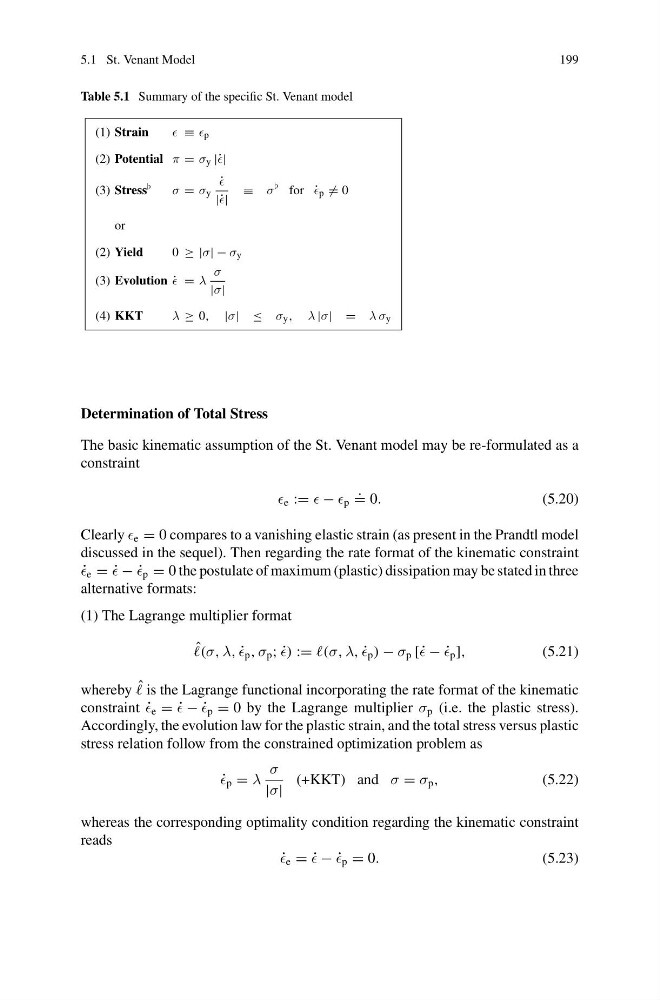
Table 5.1 Summary of the specific St. Venant model
(1) Strain
≡ p
(2) Potential π = σ y |˙ |
(3) Stress
σ = σ y
˙
|˙ |
≡ σ
for ˙
p = 0
or
(2) Yield
0 ≥ |σ| − σ y
(3) Evolution ˙
= λ
σ
|σ|
(4) KKT
λ ≥ 0, |σ| ≤ σ y , λ |σ| = λ σ y
Determination of Total Stress
The basic kinematic assumption of the St. Venant model may be re-formulated as a
constraint
e := − p
.
= 0.
(5.20)
Clearly e = 0 compares to a vanishing elastic strain (as present in the Prandtl model
discussed in the sequel). Then regarding the rate format of the kinematic constraint
˙
e = ˙
− ˙
p = 0 the postulate of maximum (plastic) dissipation may be stated in three
alternative formats:
(1) The Lagrange multiplier format
ˆ
(σ, λ, ˙
p , σ p ; ˙
) := (σ, λ, ˙
p ) − σ p [˙ − ˙
p ],
(5.21)
whereby ˆ
is the Lagrange functional incorporating the rate format of the kinematic
constraint ˙
e = ˙
− ˙
p = 0 by the Lagrange multiplier σ p (i.e. the plastic stress).
Accordingly, the evolution law for the plastic strain, and the total stress versus plastic
stress relation follow from the constrained optimization problem as
˙
p = λ
σ
|σ|
(+KKT) and σ = σ p ,
(5.22)
whereas the corresponding optimality condition regarding the kinematic constraint
reads
˙
e = ˙
− ˙
p = 0.
(5.23)
199
Table 5.1 Summary of the specific St. Venant model
(1) Strain
≡ p
(2) Potential π = σ y |˙ |
(3) Stress
σ = σ y
˙
|˙ |
≡ σ
for ˙
p = 0
or
(2) Yield
0 ≥ |σ| − σ y
(3) Evolution ˙
= λ
σ
|σ|
(4) KKT
λ ≥ 0, |σ| ≤ σ y , λ |σ| = λ σ y
Determination of Total Stress
The basic kinematic assumption of the St. Venant model may be re-formulated as a
constraint
e := − p
.
= 0.
(5.20)
Clearly e = 0 compares to a vanishing elastic strain (as present in the Prandtl model
discussed in the sequel). Then regarding the rate format of the kinematic constraint
˙
e = ˙
− ˙
p = 0 the postulate of maximum (plastic) dissipation may be stated in three
alternative formats:
(1) The Lagrange multiplier format
ˆ
(σ, λ, ˙
p , σ p ; ˙
) := (σ, λ, ˙
p ) − σ p [˙ − ˙
p ],
(5.21)
whereby ˆ
is the Lagrange functional incorporating the rate format of the kinematic
constraint ˙
e = ˙
− ˙
p = 0 by the Lagrange multiplier σ p (i.e. the plastic stress).
Accordingly, the evolution law for the plastic strain, and the total stress versus plastic
stress relation follow from the constrained optimization problem as
˙
p = λ
σ
|σ|
(+KKT) and σ = σ p ,
(5.22)
whereas the corresponding optimality condition regarding the kinematic constraint
reads
˙
e = ˙
− ˙
p = 0.
(5.23)