

106
4 Visco-Elasticity
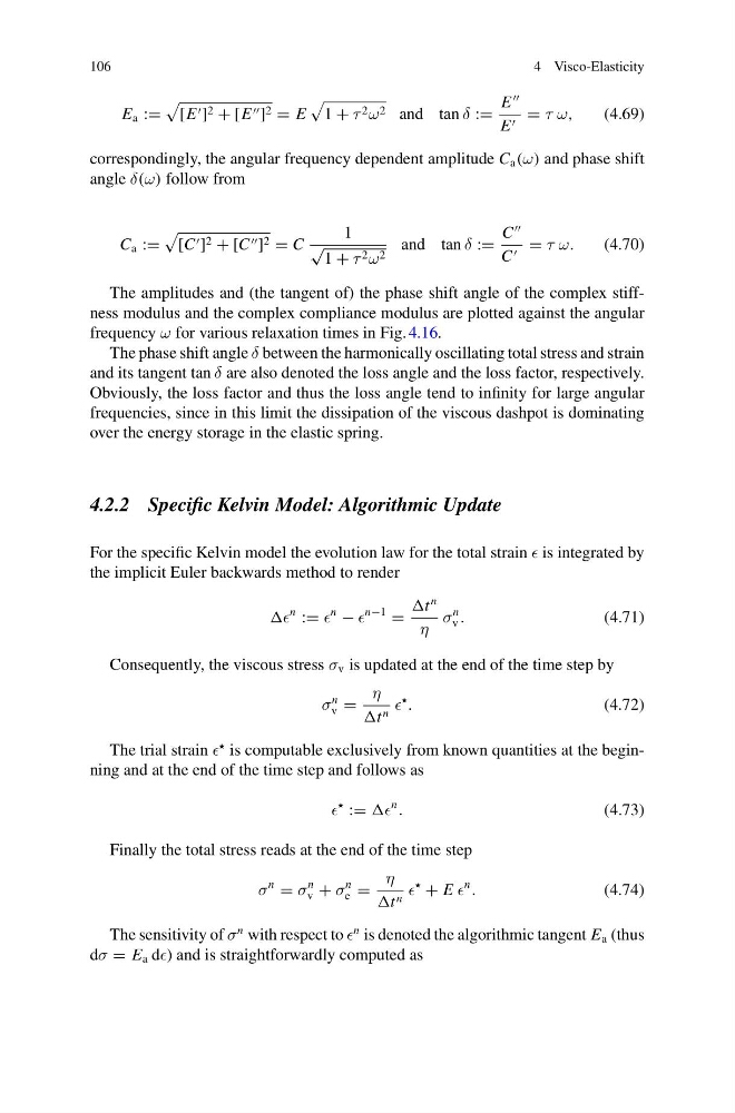
E a :=
[E ] 2 + [E ] 2 = E
1 + τ 2 ω 2 and tan δ :=
E
E = τ ω,
(4.69)
correspondingly, the angular frequency dependent amplitude C a (ω) and phase shift
angle δ(ω) follow from
C a :=
[C ] 2 + [C ] 2 = C
1
√
1 + τ 2 ω 2
and tan δ :=
C
C = τ ω.
(4.70)
The amplitudes and (the tangent of) the phase shift angle of the complex stiffness modulus and the complex compliance modulus are plotted against the angular
frequency ω for various relaxation times in Fig. 4.16.
The phase shift angle δ between the harmonically oscillating total stress and strain
and its tangent tan δ are also denoted the loss angle and the loss factor, respectively.
Obviously, the loss factor and thus the loss angle tend to infinity for large angular
frequencies, since in this limit the dissipation of the viscous dashpot is dominating
over the energy storage in the elastic spring.
4.2.2 Specific Kelvin Model: Algorithmic Update
For the specific Kelvin model the evolution law for the total strain is integrated by
the implicit Euler backwards method to render
n
:=
n
−
n−1
=
t
n
η
σ
n
v .
(4.71)
Consequently, the viscous stress σ v is updated at the end of the time step by
σ
n
v =
η
t n
.
(4.72)
The trial strain
is computable exclusively from known quantities at the beginning and at the end of the time step and follows as
:=
n
.
(4.73)
Finally the total stress reads at the end of the time step
σ
n
= σ
n
v + σ
n
e =
η
t n
+ E
n
.
(4.74)
The sensitivity of σ
n with respect to
n is denoted the algorithmic tangent E a (thus
dσ = E a d) and is straightforwardly computed as
4 Visco-Elasticity
E a :=
[E ] 2 + [E ] 2 = E
1 + τ 2 ω 2 and tan δ :=
E
E = τ ω,
(4.69)
correspondingly, the angular frequency dependent amplitude C a (ω) and phase shift
angle δ(ω) follow from
C a :=
[C ] 2 + [C ] 2 = C
1
√
1 + τ 2 ω 2
and tan δ :=
C
C = τ ω.
(4.70)
The amplitudes and (the tangent of) the phase shift angle of the complex stiffness modulus and the complex compliance modulus are plotted against the angular
frequency ω for various relaxation times in Fig. 4.16.
The phase shift angle δ between the harmonically oscillating total stress and strain
and its tangent tan δ are also denoted the loss angle and the loss factor, respectively.
Obviously, the loss factor and thus the loss angle tend to infinity for large angular
frequencies, since in this limit the dissipation of the viscous dashpot is dominating
over the energy storage in the elastic spring.
4.2.2 Specific Kelvin Model: Algorithmic Update
For the specific Kelvin model the evolution law for the total strain is integrated by
the implicit Euler backwards method to render
n
:=
n
−
n−1
=
t
n
η
σ
n
v .
(4.71)
Consequently, the viscous stress σ v is updated at the end of the time step by
σ
n
v =
η
t n
.
(4.72)
The trial strain
is computable exclusively from known quantities at the beginning and at the end of the time step and follows as
:=
n
.
(4.73)
Finally the total stress reads at the end of the time step
σ
n
= σ
n
v + σ
n
e =
η
t n
+ E
n
.
(4.74)
The sensitivity of σ
n with respect to
n is denoted the algorithmic tangent E a (thus
dσ = E a d) and is straightforwardly computed as