

5.2 Langevin Equation for the Rotor
67
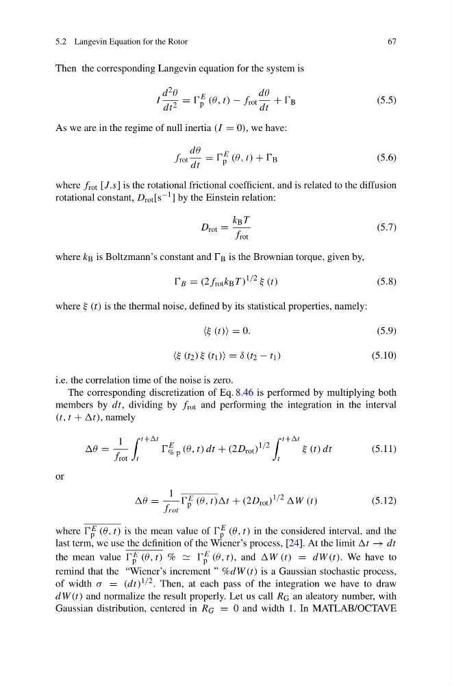
Then the corresponding Langevin equation for the system is
I
d 2 θ
dt 2 =
E
p (θ, t) − f rot
dθ
dt
+ B
(5.5)
As we are in the regime of null inertia (I = 0), we have:
f rot
dθ
dt
=
E
p (θ, t) + B
(5.6)
where f rot [J.s] is the rotational frictional coefficient, and is related to the diffusion
rotational constant, D rot [s −1 ] by the Einstein relation:
D rot =
k B T
f rot
(5.7)
where k B is Boltzmann’s constant and B is the Brownian torque, given by,
B = (2f rot k B T )
1/2 ξ (t)
(5.8)
where ξ (t) is the thermal noise, defined by its statistical properties, namely:
ξ (t) = 0.
(5.9)
ξ (t 2 ) ξ (t 1 ) = δ (t 2 − t 1 )
(5.10)
i.e. the correlation time of the noise is zero.
The corresponding discretization of Eq. 8.46 is performed by multiplying both
members by dt, dividing by f rot and performing the integration in the interval
(t, t + t), namely
θ =
1
f rot
t+t
t
E
% p (θ, t) dt + (2D rot )
1/2
t+t
t
ξ (t) dt
(5.11)
or
θ =
1
f rot
E
p (θ, t)t + (2D rot )
1/2 W (t)
(5.12)
where E
p (θ, t) is the mean value of E
p (θ, t) in the considered interval, and the
last term, we use the definition of the Wiener’s process, [24]. At the limit t → dt
the mean value E
p (θ, t) % E
p (θ, t), and W (t) = dW (t). We have to
remind that the “Wiener’s increment ” %dW (t) is a Gaussian stochastic process,
of width σ = (dt) 1/2 . Then, at each pass of the integration we have to draw
dW (t) and normalize the result properly. Let us call R G an aleatory number, with
Gaussian distribution, centered in R G = 0 and width 1. In MATLAB/OCTAVE
67
Then the corresponding Langevin equation for the system is
I
d 2 θ
dt 2 =
E
p (θ, t) − f rot
dθ
dt
+ B
(5.5)
As we are in the regime of null inertia (I = 0), we have:
f rot
dθ
dt
=
E
p (θ, t) + B
(5.6)
where f rot [J.s] is the rotational frictional coefficient, and is related to the diffusion
rotational constant, D rot [s −1 ] by the Einstein relation:
D rot =
k B T
f rot
(5.7)
where k B is Boltzmann’s constant and B is the Brownian torque, given by,
B = (2f rot k B T )
1/2 ξ (t)
(5.8)
where ξ (t) is the thermal noise, defined by its statistical properties, namely:
ξ (t) = 0.
(5.9)
ξ (t 2 ) ξ (t 1 ) = δ (t 2 − t 1 )
(5.10)
i.e. the correlation time of the noise is zero.
The corresponding discretization of Eq. 8.46 is performed by multiplying both
members by dt, dividing by f rot and performing the integration in the interval
(t, t + t), namely
θ =
1
f rot
t+t
t
E
% p (θ, t) dt + (2D rot )
1/2
t+t
t
ξ (t) dt
(5.11)
or
θ =
1
f rot
E
p (θ, t)t + (2D rot )
1/2 W (t)
(5.12)
where E
p (θ, t) is the mean value of E
p (θ, t) in the considered interval, and the
last term, we use the definition of the Wiener’s process, [24]. At the limit t → dt
the mean value E
p (θ, t) % E
p (θ, t), and W (t) = dW (t). We have to
remind that the “Wiener’s increment ” %dW (t) is a Gaussian stochastic process,
of width σ = (dt) 1/2 . Then, at each pass of the integration we have to draw
dW (t) and normalize the result properly. Let us call R G an aleatory number, with
Gaussian distribution, centered in R G = 0 and width 1. In MATLAB/OCTAVE