

66
5 Rotation of a Dipole
In Ref. [17], was shown that colloidal suspension of ferromagnetic nanoparticles,
so-called ferrofluids, are ideal systems to test theoretical predictions on fluctuation
driven transport experimentally.
Here we consider one of the simplest rotors in nature: a dipole in a viscous
medium under the influence of an oscillating electric field and thermal noise.
By applying the Langevin equation we observe rotation for some values of the
parameters.
5.2 Langevin Equation for the Rotor
The energy of a dipole in an electric field is given by
W
E
p = − −
p.
E(t) = −pE(t) cos θ
(5.1)
where |
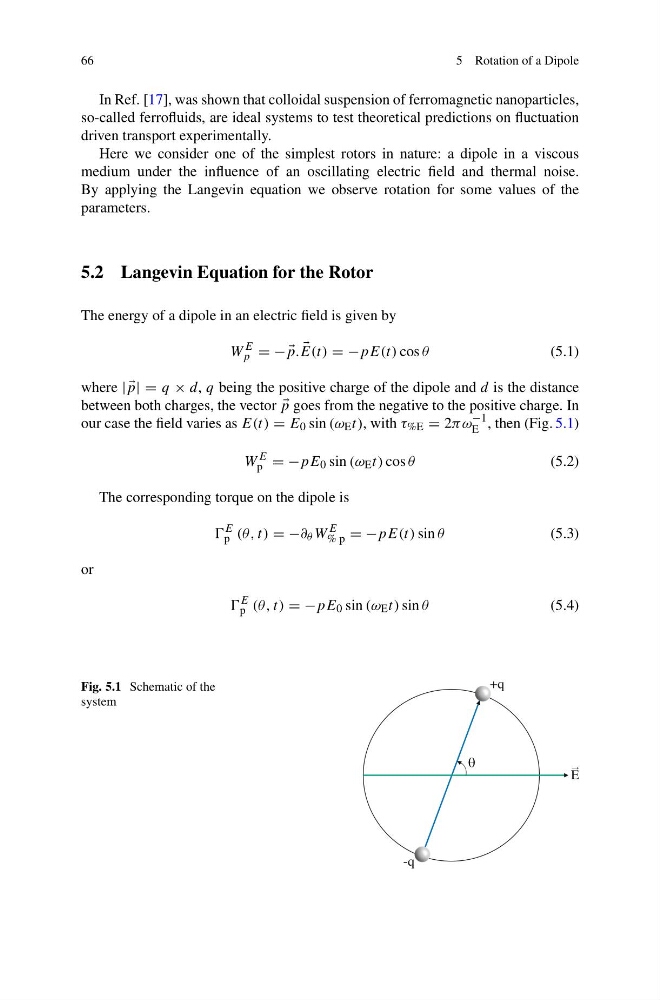
p| = q × d, q being the positive charge of the dipole and d is the distance
between both charges, the vector
p goes from the negative to the positive charge. In
our case the field varies as E(t) = E 0 sin (ω E t), with τ %E = 2πω
−1
E , then (Fig. 5.1)
W
E
p = −pE 0 sin (ω E t) cos θ
(5.2)
The corresponding torque on the dipole is
E
p (θ, t) = −∂ θ W
E
% p = −pE(t) sin θ
(5.3)
or
E
p (θ, t) = −pE 0 sin (ω E t) sin θ
(5.4)
Fig. 5.1 Schematic of the
system
5 Rotation of a Dipole
In Ref. [17], was shown that colloidal suspension of ferromagnetic nanoparticles,
so-called ferrofluids, are ideal systems to test theoretical predictions on fluctuation
driven transport experimentally.
Here we consider one of the simplest rotors in nature: a dipole in a viscous
medium under the influence of an oscillating electric field and thermal noise.
By applying the Langevin equation we observe rotation for some values of the
parameters.
5.2 Langevin Equation for the Rotor
The energy of a dipole in an electric field is given by
W
E
p = − −
p.
E(t) = −pE(t) cos θ
(5.1)
where |
p| = q × d, q being the positive charge of the dipole and d is the distance
between both charges, the vector
p goes from the negative to the positive charge. In
our case the field varies as E(t) = E 0 sin (ω E t), with τ %E = 2πω
−1
E , then (Fig. 5.1)
W
E
p = −pE 0 sin (ω E t) cos θ
(5.2)
The corresponding torque on the dipole is
E
p (θ, t) = −∂ θ W
E
% p = −pE(t) sin θ
(5.3)
or
E
p (θ, t) = −pE 0 sin (ω E t) sin θ
(5.4)
Fig. 5.1 Schematic of the
system