

68
5 Rotation of a Dipole
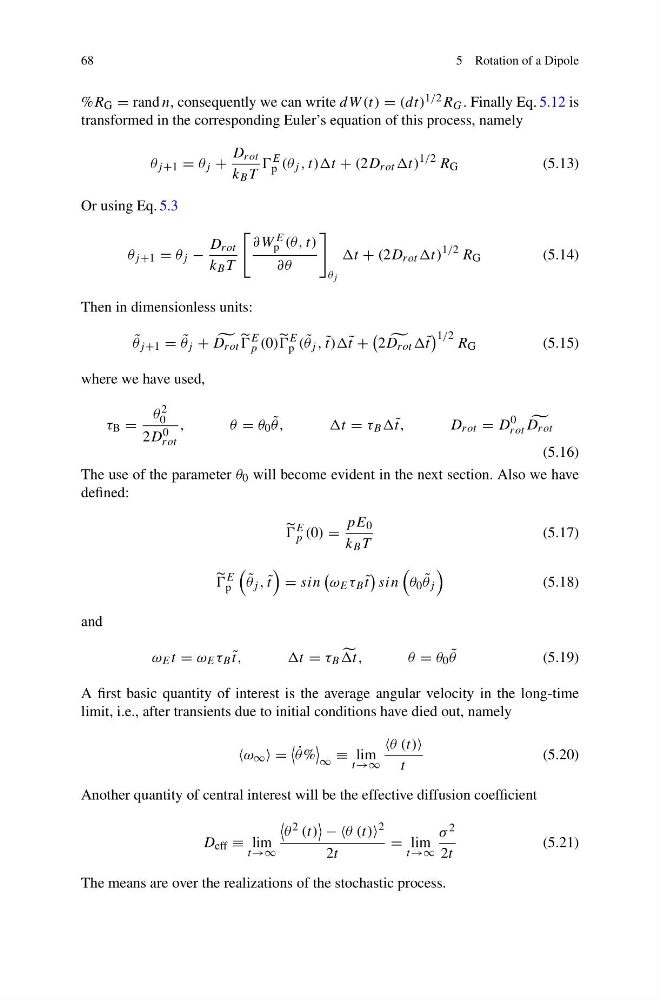
%R G = rand n, consequently we can write dW (t) = (dt) 1/2 R G . Finally Eq. 5.12 is
transformed in the corresponding Euler’s equation of this process, namely
θ j +1 = θ j +
D rot
k B T
E
p (θ j , t))t + (2D rot t)
1/2 R G
(5.13)
Or using Eq. 5.3
θ j +1 = θ j −
D rot
k B T
∂W E
p (θ, t)
∂θ
θ j
t + (2D rot t)
1/2 R G
(5.14)
Then in dimensionless units:
˜
θ j +1 = ˜
θ j +
D rot
E
p (0)
E
p ( ˜
θ j , ˜
t))˜ t +
2
D rot ˜ t
1/2 R G
(5.15)
where we have used,
τ B =
θ 2
0
2D 0
rot
,
θ= θ 0 ˜
θ,
,t = τ B ˜ t,
D rot = D
0
rot
D rot
(5.16)
The use of the parameter θ 0 will become evident in the next section. Also we have
defined:
E
p (0) =
pE 0
k B T
(5.17)
E
p
˜
θ j , ˜
t
= sin
ω E τ B ˜
t
sin
θ 0 ˜
θ j
(5.18)
and
ω E t = ω E τ B ˜
t,
,t = τ B
t,
θ = θ 0 ˜
θ
(5.19)
A first basic quantity of interest is the average angular velocity in the long-time
limit, i.e., after transients due to initial conditions have died out, namely
ω ∞ =
˙
θ %
∞
≡ lim
t→∞
θ (t)
t
(5.20)
Another quantity of central interest will be the effective diffusion coefficient
D eff ≡ lim
t→∞
θ 2 (t)
− θ (t)
2
2t
= lim
t→∞
σ 2
2t
(5.21)
The means are over the realizations of the stochastic process.
5 Rotation of a Dipole
%R G = rand n, consequently we can write dW (t) = (dt) 1/2 R G . Finally Eq. 5.12 is
transformed in the corresponding Euler’s equation of this process, namely
θ j +1 = θ j +
D rot
k B T
E
p (θ j , t))t + (2D rot t)
1/2 R G
(5.13)
Or using Eq. 5.3
θ j +1 = θ j −
D rot
k B T
∂W E
p (θ, t)
∂θ
θ j
t + (2D rot t)
1/2 R G
(5.14)
Then in dimensionless units:
˜
θ j +1 = ˜
θ j +
D rot
E
p (0)
E
p ( ˜
θ j , ˜
t))˜ t +
2
D rot ˜ t
1/2 R G
(5.15)
where we have used,
τ B =
θ 2
0
2D 0
rot
,
θ= θ 0 ˜
θ,
,t = τ B ˜ t,
D rot = D
0
rot
D rot
(5.16)
The use of the parameter θ 0 will become evident in the next section. Also we have
defined:
E
p (0) =
pE 0
k B T
(5.17)
E
p
˜
θ j , ˜
t
= sin
ω E τ B ˜
t
sin
θ 0 ˜
θ j
(5.18)
and
ω E t = ω E τ B ˜
t,
,t = τ B
t,
θ = θ 0 ˜
θ
(5.19)
A first basic quantity of interest is the average angular velocity in the long-time
limit, i.e., after transients due to initial conditions have died out, namely
ω ∞ =
˙
θ %
∞
≡ lim
t→∞
θ (t)
t
(5.20)
Another quantity of central interest will be the effective diffusion coefficient
D eff ≡ lim
t→∞
θ 2 (t)
− θ (t)
2
2t
= lim
t→∞
σ 2
2t
(5.21)
The means are over the realizations of the stochastic process.