

20
2 The Fokker-Planck Equation
M =
⎛
⎜
⎜
⎜
⎜
⎜
⎜
⎜
⎝
b c
... 0
d b c
... 0
0 d b c ... 0
. . .
. . .
0 0 0 . . . d b
⎞
⎟
⎟
⎟
⎟
⎟
⎟
⎟
⎠
P
n
=
⎛
⎜
⎜
⎜
⎜
⎜
⎜
⎜
⎝
P n
1
P n
2
P n
3
.
.
P n
N
⎞
⎟
⎟
⎟
⎟
⎟
⎟
⎟
⎠
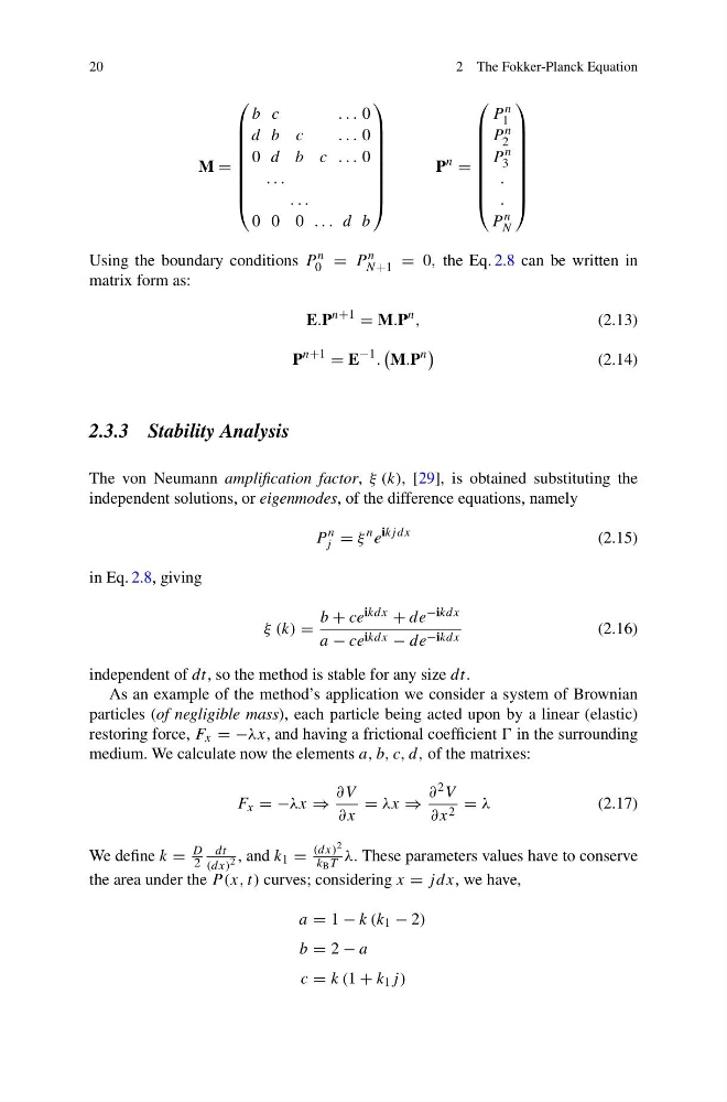
Using the boundary conditions P n
0 = P n
N +1 = 0, the Eq. 2.8 can be written in
matrix form as:
E.P
n+1
= M.P
n ,
(2.13)
P
n+1
= E
−1 .
M.P
n
(2.14)
2.3.3 Stability Analysis
The von Neumann amplification factor, ξ (k), [29], is obtained substituting the
independent solutions, or eigenmodes, of the difference equations, namely
P
n
j = ξ
n e
ikj dx
(2.15)
in Eq. 2.8, giving
ξ (k) =
b + ce ikdx + de −ikdx
a − ce ikdx − de −ikdx
(2.16)
independent of dt, so the method is stable for any size dt.
As an example of the method’s application we consider a system of Brownian
particles (of negligible mass), each particle being acted upon by a linear (elastic)
restoring force, F x = −λx, and having a frictional coefficient in the surrounding
medium. We calculate now the elements a, b, c, d, of the matrixes:
F x = −λx ⇒
∂V
∂x
= λx ⇒
∂ 2 V
∂x 2 = λ
(2.17)
We define k =
D
2
dt
(dx) 2 , and k 1 =
(dx) 2
k B T λ. These parameters values have to conserve
the area under the P (x, t) curves; considering x = jdx, we have,
a = 1 − k (k 1 − 2)
b = 2 − a
c = k (1 + k 1 j )
2 The Fokker-Planck Equation
M =
⎛
⎜
⎜
⎜
⎜
⎜
⎜
⎜
⎝
b c
... 0
d b c
... 0
0 d b c ... 0
. . .
. . .
0 0 0 . . . d b
⎞
⎟
⎟
⎟
⎟
⎟
⎟
⎟
⎠
P
n
=
⎛
⎜
⎜
⎜
⎜
⎜
⎜
⎜
⎝
P n
1
P n
2
P n
3
.
.
P n
N
⎞
⎟
⎟
⎟
⎟
⎟
⎟
⎟
⎠
Using the boundary conditions P n
0 = P n
N +1 = 0, the Eq. 2.8 can be written in
matrix form as:
E.P
n+1
= M.P
n ,
(2.13)
P
n+1
= E
−1 .
M.P
n
(2.14)
2.3.3 Stability Analysis
The von Neumann amplification factor, ξ (k), [29], is obtained substituting the
independent solutions, or eigenmodes, of the difference equations, namely
P
n
j = ξ
n e
ikj dx
(2.15)
in Eq. 2.8, giving
ξ (k) =
b + ce ikdx + de −ikdx
a − ce ikdx − de −ikdx
(2.16)
independent of dt, so the method is stable for any size dt.
As an example of the method’s application we consider a system of Brownian
particles (of negligible mass), each particle being acted upon by a linear (elastic)
restoring force, F x = −λx, and having a frictional coefficient in the surrounding
medium. We calculate now the elements a, b, c, d, of the matrixes:
F x = −λx ⇒
∂V
∂x
= λx ⇒
∂ 2 V
∂x 2 = λ
(2.17)
We define k =
D
2
dt
(dx) 2 , and k 1 =
(dx) 2
k B T λ. These parameters values have to conserve
the area under the P (x, t) curves; considering x = jdx, we have,
a = 1 − k (k 1 − 2)
b = 2 − a
c = k (1 + k 1 j )