

2.3 Discretization of the Fokker-Planck Equation
19
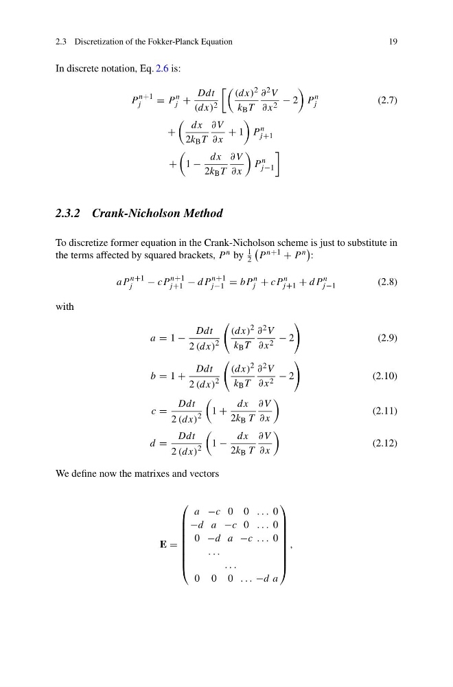
In discrete notation, Eq. 2.6 is:
P
n+1
j
= P
n
j +
Ddt
(dx) 2
(dx) 2
k B T
∂ 2 V
∂x 2 − 2
P
n
j
(2.7)
+
dx
2k B T
∂V
∂x
+ 1
P
n
j +1
+
1 −
dx
2k B T
∂V
∂x
P
n
j −1
2.3.2 Crank-Nicholson Method
To discretize former equation in the Crank-Nicholson scheme is just to substitute in
the terms affected by squared brackets, P n by
1
2
P n+1 + P n
:
aP
n+1
j
− cP
n+1
j +1 − dP
n+1
j −1 = bP
n
j + cP
n
j +1 + dP
n
j −1
(2.8)
with
a = 1 −
Ddt
2 (dx)
2
(dx)
2
k B T
∂ 2 V
∂x 2 − 2
(2.9)
b = 1 +
Ddt
2 (dx)
2
(dx)
2
k B T
∂ 2 V
∂x 2 − 2
(2.10)
c =
Ddt
2 (dx)
2
1 +
dx
2k B T
∂V
∂x
(2.11)
d =
Ddt
2 (dx)
2
1 −
dx
2k B T
∂V
∂x
(2.12)
We define now the matrixes and vectors
E =
⎛
⎜
⎜
⎜
⎜
⎜
⎜
⎜
⎝
a −c 0 0 . . . 0
−d a −c 0 . . . 0
0 −d a −c . . . 0
. . .
. . .
0 0 0 . . . −d a
⎞
⎟
⎟
⎟
⎟
⎟
⎟
⎟
⎠
,
19
In discrete notation, Eq. 2.6 is:
P
n+1
j
= P
n
j +
Ddt
(dx) 2
(dx) 2
k B T
∂ 2 V
∂x 2 − 2
P
n
j
(2.7)
+
dx
2k B T
∂V
∂x
+ 1
P
n
j +1
+
1 −
dx
2k B T
∂V
∂x
P
n
j −1
2.3.2 Crank-Nicholson Method
To discretize former equation in the Crank-Nicholson scheme is just to substitute in
the terms affected by squared brackets, P n by
1
2
P n+1 + P n
:
aP
n+1
j
− cP
n+1
j +1 − dP
n+1
j −1 = bP
n
j + cP
n
j +1 + dP
n
j −1
(2.8)
with
a = 1 −
Ddt
2 (dx)
2
(dx)
2
k B T
∂ 2 V
∂x 2 − 2
(2.9)
b = 1 +
Ddt
2 (dx)
2
(dx)
2
k B T
∂ 2 V
∂x 2 − 2
(2.10)
c =
Ddt
2 (dx)
2
1 +
dx
2k B T
∂V
∂x
(2.11)
d =
Ddt
2 (dx)
2
1 −
dx
2k B T
∂V
∂x
(2.12)
We define now the matrixes and vectors
E =
⎛
⎜
⎜
⎜
⎜
⎜
⎜
⎜
⎝
a −c 0 0 . . . 0
−d a −c 0 . . . 0
0 −d a −c . . . 0
. . .
. . .
0 0 0 . . . −d a
⎞
⎟
⎟
⎟
⎟
⎟
⎟
⎟
⎠
,