

18
2 The Fokker-Planck Equation
Integrating in x follows
1
∂V (x)
∂x
P (x) + D
∂P (x)
∂x
= constant.
As P is the equilibrium distribution, its dependency in x is given by Boltzmann
distribution, i.e.,
P (x) ∝ exp −
V (x)
k B T
2.3 Discretization of the Fokker-Planck Equation
2.3.1 Forward Time Central Space (FTCS) Method
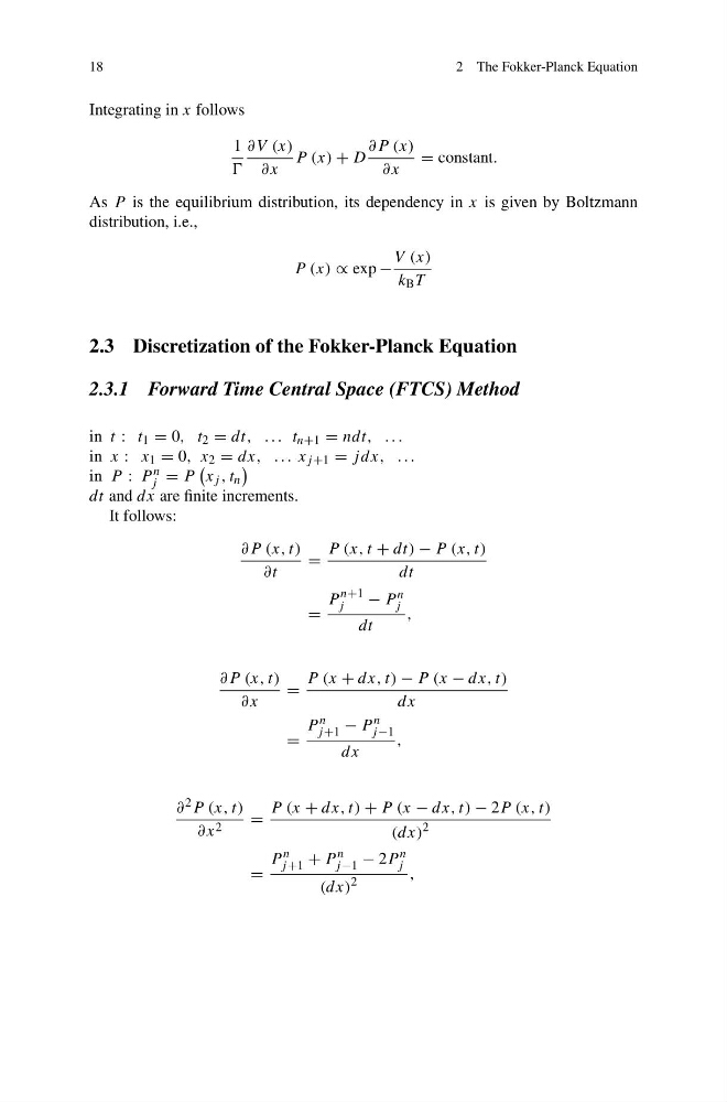
in t : t 1 = 0, t 2 = dt, . . . t n+1 = ndt, . . .
in x : x 1 = 0, x 2 = dx, . . . x j +1 = jdx, . . .
in P : P n
j = P
x j , t n
dt and dx are finite increments.
It follows:
∂P (x, t)
∂t
=
P (x, t + dt) − P (x, t)
dt
=
P
n+1
j
− P n
j
dt
,
∂P (x, t)
∂x
=
P (x + dx, t) − P (x − dx, t)
dx
=
P n
j +1 − P n
j −1
dx
,
∂ 2 P (x, t)
∂x 2
=
P (x + dx, t) + P (x − dx, t) − 2P (x, t)
(dx)
2
=
P n
j +1 + P n
j −1 − 2P n
j
(dx)
2
,
2 The Fokker-Planck Equation
Integrating in x follows
1
∂V (x)
∂x
P (x) + D
∂P (x)
∂x
= constant.
As P is the equilibrium distribution, its dependency in x is given by Boltzmann
distribution, i.e.,
P (x) ∝ exp −
V (x)
k B T
2.3 Discretization of the Fokker-Planck Equation
2.3.1 Forward Time Central Space (FTCS) Method
in t : t 1 = 0, t 2 = dt, . . . t n+1 = ndt, . . .
in x : x 1 = 0, x 2 = dx, . . . x j +1 = jdx, . . .
in P : P n
j = P
x j , t n
dt and dx are finite increments.
It follows:
∂P (x, t)
∂t
=
P (x, t + dt) − P (x, t)
dt
=
P
n+1
j
− P n
j
dt
,
∂P (x, t)
∂x
=
P (x + dx, t) − P (x − dx, t)
dx
=
P n
j +1 − P n
j −1
dx
,
∂ 2 P (x, t)
∂x 2
=
P (x + dx, t) + P (x − dx, t) − 2P (x, t)
(dx)
2
=
P n
j +1 + P n
j −1 − 2P n
j
(dx)
2
,