

2.4 Program 2.1, F-P Equation, Matlab Code
21
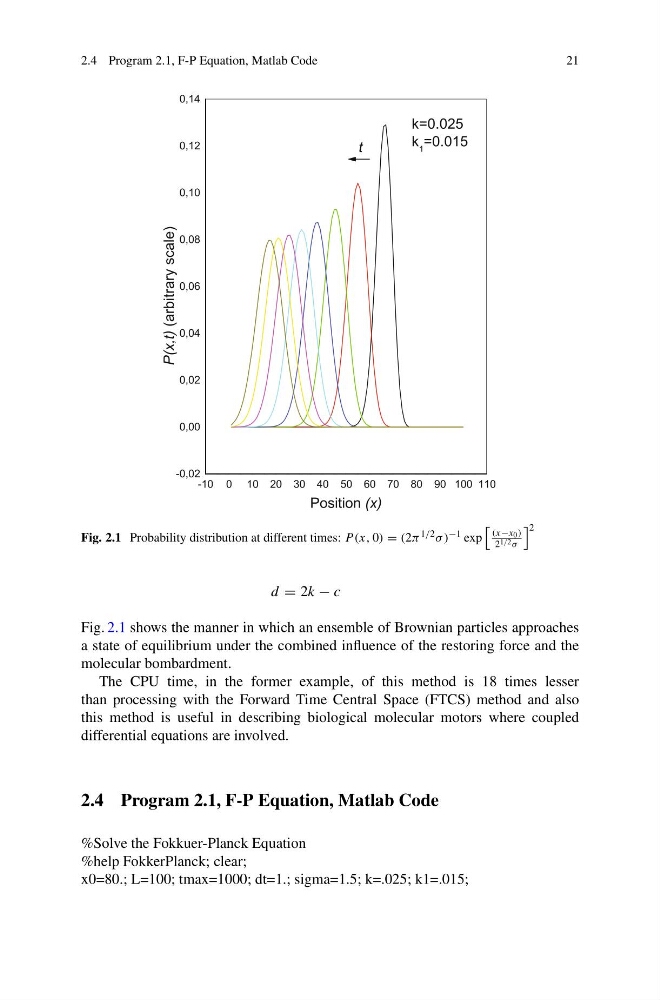
Fig. 2.1 Probability distribution at different times: P (x, 0) = (2π 1/2 σ ) −1 exp
(x−x 0 )
2 1/2 σ
2
d = 2k − c
Fig. 2.1 shows the manner in which an ensemble of Brownian particles approaches
a state of equilibrium under the combined influence of the restoring force and the
molecular bombardment.
The CPU time, in the former example, of this method is 18 times lesser
than processing with the Forward Time Central Space (FTCS) method and also
this method is useful in describing biological molecular motors where coupled
differential equations are involved.
2.4 Program 2.1, F-P Equation, Matlab Code
%Solve the Fokkuer-Planck Equation
%help FokkerPlanck; clear;
x0=80.; L=100; tmax=1000; dt=1.; sigma=1.5; k=.025; k1=.015;
21
Fig. 2.1 Probability distribution at different times: P (x, 0) = (2π 1/2 σ ) −1 exp
(x−x 0 )
2 1/2 σ
2
d = 2k − c
Fig. 2.1 shows the manner in which an ensemble of Brownian particles approaches
a state of equilibrium under the combined influence of the restoring force and the
molecular bombardment.
The CPU time, in the former example, of this method is 18 times lesser
than processing with the Forward Time Central Space (FTCS) method and also
this method is useful in describing biological molecular motors where coupled
differential equations are involved.
2.4 Program 2.1, F-P Equation, Matlab Code
%Solve the Fokkuer-Planck Equation
%help FokkerPlanck; clear;
x0=80.; L=100; tmax=1000; dt=1.; sigma=1.5; k=.025; k1=.015;