

3.1 Error Function from Statistical Mechanics
45
As can be seen from the figure, the expectation value of h gradually approaches
max(Jx + J, 0) as the number of bits increases. Let us call it σ ReLU (z) = max(z, 0),
and if we adopt the approximation, we find:
J,x[i] ≈ σ ReLU (Jx[i] + J ) ,
(3.41)
{h
(u)
bit }
Q
d[i]
h =
N bits
u=1
h
(u)
bit
Q J ({h
(u)
bit }|x[i]) ≈ Q
d[i]
h = =h J,x[i]
.
(3.42)
Furthermore, the error function is
− log Q
d[i]
h = =h J,x[i]
≈
1
2
d[i] − σ ReLU (Jx[i] + J )
2
.
(3.43)
Multi-component teaching signal
In addition to the multi-component labels as shown in Fig. 3.2, we can set d I ∈
{0, 1} or d I ∈ R. In that case, we need to consider the output of applying σ or
σ ReLU to each component.
3.1.2 Deep Neural Network
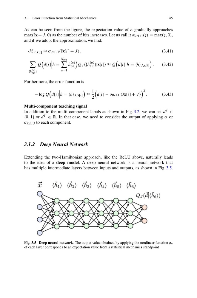
Extending the two-Hamiltonian approach, like the ReLU above, naturally leads
to the idea of a deep model. A deep neural network is a neural network that
has multiple intermediate layers between inputs and outputs, as shown in Fig. 3.5.
Fig. 3.5 Deep neural network. The output value obtained by applying the nonlinear function σ •
of each layer corresponds to an expectation value from a statistical mechanics standpoint
45
As can be seen from the figure, the expectation value of h gradually approaches
max(Jx + J, 0) as the number of bits increases. Let us call it σ ReLU (z) = max(z, 0),
and if we adopt the approximation, we find:
J,x[i] ≈ σ ReLU (Jx[i] + J ) ,
(3.41)
{h
(u)
bit }
Q
d[i]
h =
N bits
u=1
h
(u)
bit
Q J ({h
(u)
bit }|x[i]) ≈ Q
d[i]
h = =h J,x[i]
.
(3.42)
Furthermore, the error function is
− log Q
d[i]
h = =h J,x[i]
≈
1
2
d[i] − σ ReLU (Jx[i] + J )
2
.
(3.43)
Multi-component teaching signal
In addition to the multi-component labels as shown in Fig. 3.2, we can set d I ∈
{0, 1} or d I ∈ R. In that case, we need to consider the output of applying σ or
σ ReLU to each component.
3.1.2 Deep Neural Network
Extending the two-Hamiltonian approach, like the ReLU above, naturally leads
to the idea of a deep model. A deep neural network is a neural network that
has multiple intermediate layers between inputs and outputs, as shown in Fig. 3.5.
Fig. 3.5 Deep neural network. The output value obtained by applying the nonlinear function σ •
of each layer corresponds to an expectation value from a statistical mechanics standpoint