

44
3 Basics of Neural Networks
Then we find
−
x,d
P (x, d) log Q J (d|x)
≈ −
i:Data
1
The number of data
log Q J (d[i]|x[i])
=
−1
The number of data
i:Data
log
{h
(u)
bit }
Q
d[i]
h =
N bits
u=1
h
(u)
bit
Q J ({h
(u)
bit }|x[i])
(3.39)
Just as the probability mean for x, d is replaced with the data (sample from P ) mean,
let also the probability mean for {h
(u)
bit } in the log be replaced with the average under
Q J ({h
(u)
bit }|x[i]). As a test, we calculate the average of h under Q J ({h
(u)
bit }|x[i]), then
we find
J,x[i] =
{h
(u)
bit }
N bits
u=1
h
(u)
bit
Q J ({h
(u)
bit }|x[i]) =
N bits
u=1
σ (Jx + J + 0.5 − u) .
(3.40)
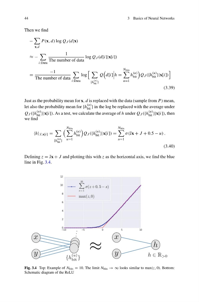
Defining z = Jx + J and plotting this with z as the horizontal axis, we find the blue
line in Fig. 3.4.
x
y
. . .
{h
(u)
bit }
x
y
h
≈
h ∈ R >0
Fig. 3.4 Top: Example of N bits = 10. The limit N bits → ∞ looks similar to max(z, 0). Bottom:
Schematic diagram of the ReLU
3 Basics of Neural Networks
Then we find
−
x,d
P (x, d) log Q J (d|x)
≈ −
i:Data
1
The number of data
log Q J (d[i]|x[i])
=
−1
The number of data
i:Data
log
{h
(u)
bit }
Q
d[i]
h =
N bits
u=1
h
(u)
bit
Q J ({h
(u)
bit }|x[i])
(3.39)
Just as the probability mean for x, d is replaced with the data (sample from P ) mean,
let also the probability mean for {h
(u)
bit } in the log be replaced with the average under
Q J ({h
(u)
bit }|x[i]). As a test, we calculate the average of h under Q J ({h
(u)
bit }|x[i]), then
we find
J,x[i] =
{h
(u)
bit }
N bits
u=1
h
(u)
bit
Q J ({h
(u)
bit }|x[i]) =
N bits
u=1
σ (Jx + J + 0.5 − u) .
(3.40)
Defining z = Jx + J and plotting this with z as the horizontal axis, we find the blue
line in Fig. 3.4.
x
y
. . .
{h
(u)
bit }
x
y
h
≈
h ∈ R >0
Fig. 3.4 Top: Example of N bits = 10. The limit N bits → ∞ looks similar to max(z, 0). Bottom:
Schematic diagram of the ReLU