

12.2 Curved Spacetime Is a Neural Network
179
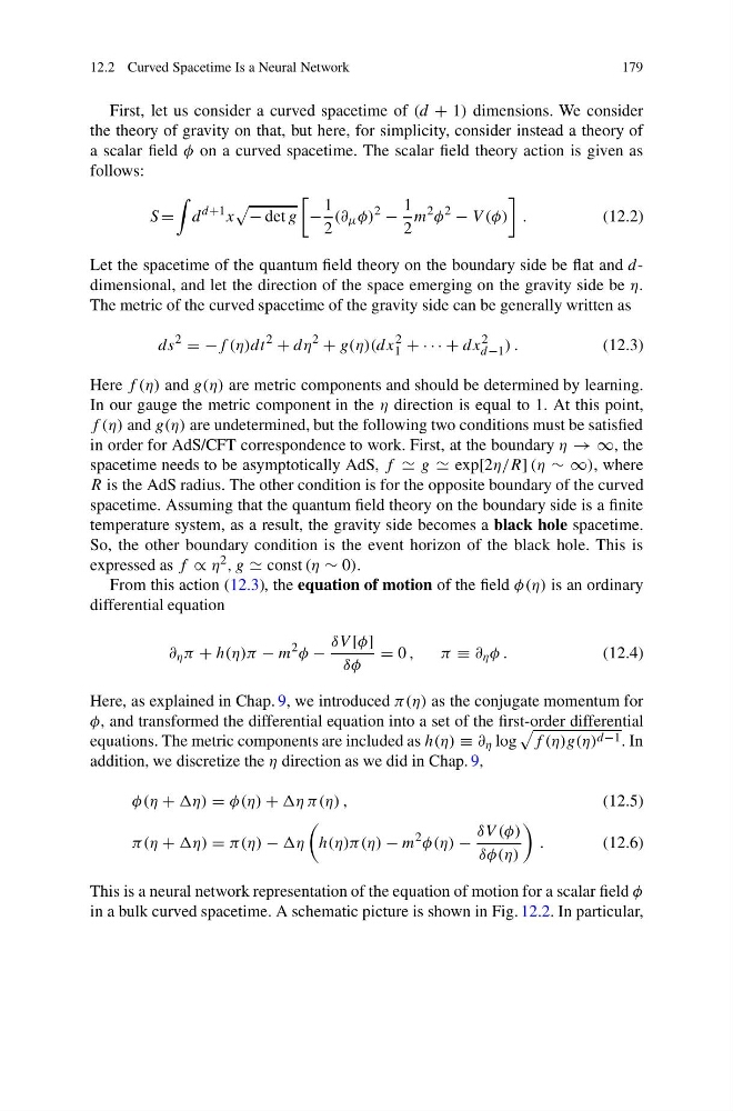
First, let us consider a curved spacetime of (d + 1) dimensions. We consider
the theory of gravity on that, but here, for simplicity, consider instead a theory of
a scalar field φ on a curved spacetime. The scalar field theory action is given as
follows:
S =
d
d+1 x
− det g
−
1
2
(∂ μ φ)
2
−
1
2
m
2 φ
2
− V (φ)
.
(12.2)
Let the spacetime of the quantum field theory on the boundary side be flat and ddimensional, and let the direction of the space emerging on the gravity side be η.
The metric of the curved spacetime of the gravity side can be generally written as
ds
2
= −f (η)dt
2
+ dη
2
+ g(η)(dx
2
1 + · · · + dx
2
d−1 ) .
(12.3)
Here f (η) and g(η) are metric components and should be determined by learning.
In our gauge the metric component in the η direction is equal to 1. At this point,
f (η) and g(η) are undetermined, but the following two conditions must be satisfied
in order for AdS/CFT correspondence to work. First, at the boundary η → ∞, the
spacetime needs to be asymptotically AdS, f g exp[2η/R] (η ∼ ∞), where
R is the AdS radius. The other condition is for the opposite boundary of the curved
spacetime. Assuming that the quantum field theory on the boundary side is a finite
temperature system, as a result, the gravity side becomes a black hole spacetime.
So, the other boundary condition is the event horizon of the black hole. This is
expressed as f ∝ η 2 , g const (η ∼ 0).
From this action (12.3), the equation of motion of the field φ(η) is an ordinary
differential equation
∂ η π + h(η)π − m
2 φ −
δV [φ]
δφ
= 0 ,
π ≡ ∂ η φ .
(12.4)
Here, as explained in Chap. 9, we introduced π(η) as the conjugate momentum for
φ, and transformed the differential equation into a set of the first-order differential
equations. The metric components are included as h(η) ≡ ∂ η log
f (η)g(η) d−1 . In
addition, we discretize the η direction as we did in Chap. 9,
φ(η + = φ(η) + η π(η) ,
(12.5)
π(η + = π(η) −
h(η)π(η) − m
2 φ(η) −
δV (φ)
δφ(η)
.
(12.6)
This is a neural network representation of the equation of motion for a scalar field φ
in a bulk curved spacetime. A schematic picture is shown in Fig. 12.2. In particular,
179
First, let us consider a curved spacetime of (d + 1) dimensions. We consider
the theory of gravity on that, but here, for simplicity, consider instead a theory of
a scalar field φ on a curved spacetime. The scalar field theory action is given as
follows:
S =
d
d+1 x
− det g
−
1
2
(∂ μ φ)
2
−
1
2
m
2 φ
2
− V (φ)
.
(12.2)
Let the spacetime of the quantum field theory on the boundary side be flat and ddimensional, and let the direction of the space emerging on the gravity side be η.
The metric of the curved spacetime of the gravity side can be generally written as
ds
2
= −f (η)dt
2
+ dη
2
+ g(η)(dx
2
1 + · · · + dx
2
d−1 ) .
(12.3)
Here f (η) and g(η) are metric components and should be determined by learning.
In our gauge the metric component in the η direction is equal to 1. At this point,
f (η) and g(η) are undetermined, but the following two conditions must be satisfied
in order for AdS/CFT correspondence to work. First, at the boundary η → ∞, the
spacetime needs to be asymptotically AdS, f g exp[2η/R] (η ∼ ∞), where
R is the AdS radius. The other condition is for the opposite boundary of the curved
spacetime. Assuming that the quantum field theory on the boundary side is a finite
temperature system, as a result, the gravity side becomes a black hole spacetime.
So, the other boundary condition is the event horizon of the black hole. This is
expressed as f ∝ η 2 , g const (η ∼ 0).
From this action (12.3), the equation of motion of the field φ(η) is an ordinary
differential equation
∂ η π + h(η)π − m
2 φ −
δV [φ]
δφ
= 0 ,
π ≡ ∂ η φ .
(12.4)
Here, as explained in Chap. 9, we introduced π(η) as the conjugate momentum for
φ, and transformed the differential equation into a set of the first-order differential
equations. The metric components are included as h(η) ≡ ∂ η log
f (η)g(η) d−1 . In
addition, we discretize the η direction as we did in Chap. 9,
φ(η + = φ(η) + η π(η) ,
(12.5)
π(η + = π(η) −
h(η)π(η) − m
2 φ(η) −
δV (φ)
δφ(η)
.
(12.6)
This is a neural network representation of the equation of motion for a scalar field φ
in a bulk curved spacetime. A schematic picture is shown in Fig. 12.2. In particular,