

180
12 Application to Superstring Theory
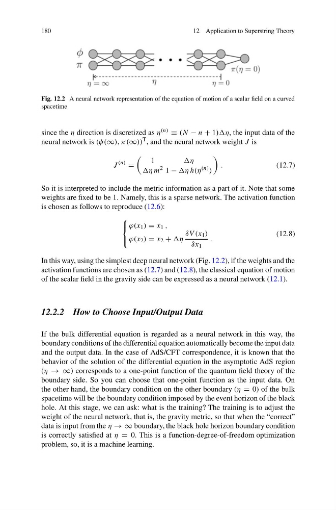
Fig. 12.2 A neural network representation of the equation of motion of a scalar field on a curved
spacetime
since the η direction is discretized as η (n) ≡ (N − n + 1))η, the input data of the
neural network is (φ(∞), π(∞)) T , and the neural network weight J is
J
(n)
=
1
η
η m 2 1 − η h(η (n) )
.
(12.7)
So it is interpreted to include the metric information as a part of it. Note that some
weights are fixed to be 1. Namely, this is a sparse network. The activation function
is chosen as follows to reproduce (12.6):
⎧
⎨
⎩
ϕ(x 1 ) = x 1 ,
ϕ(x 2 ) = x 2 + η
δV (x 1 )
δx 1
.
(12.8)
In this way, using the simplest deep neural network (Fig. 12.2), if the weights and the
activation functions are chosen as (12.7) and (12.8), the classical equation of motion
of the scalar field in the gravity side can be expressed as a neural network (12.1).
12.2.2 How to Choose Input/Output Data
If the bulk differential equation is regarded as a neural network in this way, the
boundary conditions of the differential equation automatically become the input data
and the output data. In the case of AdS/CFT correspondence, it is known that the
behavior of the solution of the differential equation in the asymptotic AdS region
(η → ∞) corresponds to a one-point function of the quantum field theory of the
boundary side. So you can choose that one-point function as the input data. On
the other hand, the boundary condition on the other boundary (η = 0) of the bulk
spacetime will be the boundary condition imposed by the event horizon of the black
hole. At this stage, we can ask: what is the training? The training is to adjust the
weight of the neural network, that is, the gravity metric, so that when the “correct”
data is input from the η → ∞ boundary, the black hole horizon boundary condition
is correctly satisfied at η = 0. This is a function-degree-of-freedom optimization
problem, so, it is a machine learning.
12 Application to Superstring Theory
Fig. 12.2 A neural network representation of the equation of motion of a scalar field on a curved
spacetime
since the η direction is discretized as η (n) ≡ (N − n + 1))η, the input data of the
neural network is (φ(∞), π(∞)) T , and the neural network weight J is
J
(n)
=
1
η
η m 2 1 − η h(η (n) )
.
(12.7)
So it is interpreted to include the metric information as a part of it. Note that some
weights are fixed to be 1. Namely, this is a sparse network. The activation function
is chosen as follows to reproduce (12.6):
⎧
⎨
⎩
ϕ(x 1 ) = x 1 ,
ϕ(x 2 ) = x 2 + η
δV (x 1 )
δx 1
.
(12.8)
In this way, using the simplest deep neural network (Fig. 12.2), if the weights and the
activation functions are chosen as (12.7) and (12.8), the classical equation of motion
of the scalar field in the gravity side can be expressed as a neural network (12.1).
12.2.2 How to Choose Input/Output Data
If the bulk differential equation is regarded as a neural network in this way, the
boundary conditions of the differential equation automatically become the input data
and the output data. In the case of AdS/CFT correspondence, it is known that the
behavior of the solution of the differential equation in the asymptotic AdS region
(η → ∞) corresponds to a one-point function of the quantum field theory of the
boundary side. So you can choose that one-point function as the input data. On
the other hand, the boundary condition on the other boundary (η = 0) of the bulk
spacetime will be the boundary condition imposed by the event horizon of the black
hole. At this stage, we can ask: what is the training? The training is to adjust the
weight of the neural network, that is, the gravity metric, so that when the “correct”
data is input from the η → ∞ boundary, the black hole horizon boundary condition
is correctly satisfied at η = 0. This is a function-degree-of-freedom optimization
problem, so, it is a machine learning.