

108
6 Unsupervised Deep Learning
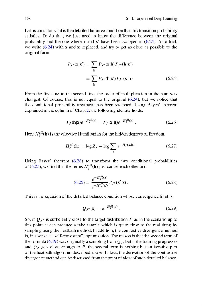
Let us consider what is the detailed balance condition that this transition probability
satisfies. To do that, we just need to know the difference between the original
probability and the one where x and x have been swapped in (6.24). As a trial,
we write (6.24) with x and x replaced, and try to get as close as possible to the
original form:
P J ∗ (x|x
) =
h
P J ∗ (x|h)P J ∗ (h|x
)
=
h
P J ∗ (h|x
)P J ∗ (x|h) .
(6.25)
From the first line to the second line, the order of multiplication in the sum was
changed. Of course, this is not equal to the original (6.24), but we notice that
the conditional probability argument has been swapped. Using Bayes’ theorem
explained in the column of Chap. 2, the following identity holds:
P J (h|x)e
−H eff
J (x)
= P J (x|h)e
−H eff
J (h) .
(6.26)
Here H eff
J (h) is the effective Hamiltonian for the hidden degrees of freedom,
H
eff
J (h) = log Z J − log
x
e
−H J (x,h) .
(6.27)
Using Bayes’ theorem (6.26) to transform the two conditional probabilities
of (6.25), we find that the terms H
eff
J (h) just cancel each other and
(6.25) =
e
−H eff
J ∗ (x)
e
−H eff
J ∗ (x )
P J ∗ (x
|x) .
(6.28)
This is the equation of the detailed balance condition whose convergence limit is
Q J ∗ (x) = e
−H eff
J ∗ (x) .
(6.29)
So, if Q J ∗ is sufficiently close to the target distribution P as in the scenario up to
this point, it can produce a fake sample which is quite close to the real thing by
sampling using the heatbath method. In addition, the contrastive divergence method
is, in a sense, a “self-consistent” ˙ I optimization. The reason is that the second term of
the formula (6.19) was originally a sampling from Q J , but if the training progresses
and Q J gets close enough to P , the second term is nothing but an iterative part
of the heatbath algorithm described above. In fact, the derivation of the contrastive
divergence method can be discussed from the point of view of such detailed balance.
6 Unsupervised Deep Learning
Let us consider what is the detailed balance condition that this transition probability
satisfies. To do that, we just need to know the difference between the original
probability and the one where x and x have been swapped in (6.24). As a trial,
we write (6.24) with x and x replaced, and try to get as close as possible to the
original form:
P J ∗ (x|x
) =
h
P J ∗ (x|h)P J ∗ (h|x
)
=
h
P J ∗ (h|x
)P J ∗ (x|h) .
(6.25)
From the first line to the second line, the order of multiplication in the sum was
changed. Of course, this is not equal to the original (6.24), but we notice that
the conditional probability argument has been swapped. Using Bayes’ theorem
explained in the column of Chap. 2, the following identity holds:
P J (h|x)e
−H eff
J (x)
= P J (x|h)e
−H eff
J (h) .
(6.26)
Here H eff
J (h) is the effective Hamiltonian for the hidden degrees of freedom,
H
eff
J (h) = log Z J − log
x
e
−H J (x,h) .
(6.27)
Using Bayes’ theorem (6.26) to transform the two conditional probabilities
of (6.25), we find that the terms H
eff
J (h) just cancel each other and
(6.25) =
e
−H eff
J ∗ (x)
e
−H eff
J ∗ (x )
P J ∗ (x
|x) .
(6.28)
This is the equation of the detailed balance condition whose convergence limit is
Q J ∗ (x) = e
−H eff
J ∗ (x) .
(6.29)
So, if Q J ∗ is sufficiently close to the target distribution P as in the scenario up to
this point, it can produce a fake sample which is quite close to the real thing by
sampling using the heatbath method. In addition, the contrastive divergence method
is, in a sense, a “self-consistent” ˙ I optimization. The reason is that the second term of
the formula (6.19) was originally a sampling from Q J , but if the training progresses
and Q J gets close enough to P , the second term is nothing but an iterative part
of the heatbath algorithm described above. In fact, the derivation of the contrastive
divergence method can be discussed from the point of view of such detailed balance.