

6.2 Boltzmann Machine
107
Training of a restricted Boltzmann machine
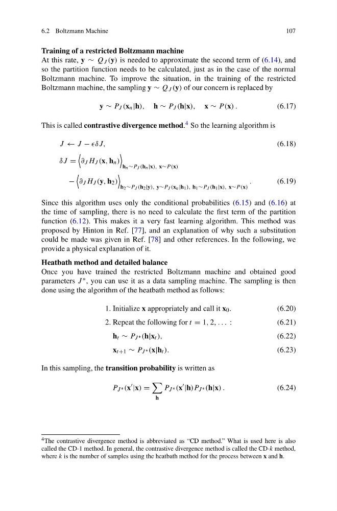
At this rate, y ∼ Q J (y) is needed to approximate the second term of (6.14), and
so the partition function needs to be calculated, just as in the case of the normal
Boltzmann machine. To improve the situation, in the training of the restricted
Boltzmann machine, the sampling y ∼ Q J (y) of our concern is replaced by
y ∼ P J (x n |h), h ∼ P J (h|x), x ∼ P (x) .
(6.17)
This is called contrastive divergence method. 4 So the learning algorithm is
J ← J − δJ,
(6.18)
δJ =
∂ J H J (x, h n )
h n ∼P J (h n |x), x∼P (x)
−
∂ J H J (y, h 2 )
h 2 ∼P J (h 2 |y), y∼P J (x n |h 1 ), h 1 ∼P J (h 1 |x), x∼P (x)
.
(6.19)
Since this algorithm uses only the conditional probabilities (6.15) and (6.16) at
the time of sampling, there is no need to calculate the first term of the partition
function (6.12). This makes it a very fast learning algorithm. This method was
proposed by Hinton in Ref. [77], and an explanation of why such a substitution
could be made was given in Ref. [78] and other references. In the following, we
provide a physical explanation of it.
Heatbath method and detailed balance
Once you have trained the restricted Boltzmann machine and obtained good
parameters J ∗ , you can use it as a data sampling machine. The sampling is then
done using the algorithm of the heatbath method as follows:
1. Initialize x appropriately and call it x 0 .
(6.20)
2. Repeat the following for t = 1, 2, . . . :
(6.21)
h t ∼ P J ∗ (h|x t ),
(6.22)
x t +1 ∼ P J ∗ (x|h t ).
(6.23)
In this sampling, the transition probability is written as
P J ∗ (x
|x) =
h
P J ∗ (x
|h)P J ∗ (h|x) .
(6.24)
4 The contrastive divergence method is abbreviated as “CD method.” What is used here is also
called the CD-1 method. In general, the contrastive divergence method is called the CD-k method,
where k is the number of samples using the heatbath method for the process between x and h.
107
Training of a restricted Boltzmann machine
At this rate, y ∼ Q J (y) is needed to approximate the second term of (6.14), and
so the partition function needs to be calculated, just as in the case of the normal
Boltzmann machine. To improve the situation, in the training of the restricted
Boltzmann machine, the sampling y ∼ Q J (y) of our concern is replaced by
y ∼ P J (x n |h), h ∼ P J (h|x), x ∼ P (x) .
(6.17)
This is called contrastive divergence method. 4 So the learning algorithm is
J ← J − δJ,
(6.18)
δJ =
∂ J H J (x, h n )
h n ∼P J (h n |x), x∼P (x)
−
∂ J H J (y, h 2 )
h 2 ∼P J (h 2 |y), y∼P J (x n |h 1 ), h 1 ∼P J (h 1 |x), x∼P (x)
.
(6.19)
Since this algorithm uses only the conditional probabilities (6.15) and (6.16) at
the time of sampling, there is no need to calculate the first term of the partition
function (6.12). This makes it a very fast learning algorithm. This method was
proposed by Hinton in Ref. [77], and an explanation of why such a substitution
could be made was given in Ref. [78] and other references. In the following, we
provide a physical explanation of it.
Heatbath method and detailed balance
Once you have trained the restricted Boltzmann machine and obtained good
parameters J ∗ , you can use it as a data sampling machine. The sampling is then
done using the algorithm of the heatbath method as follows:
1. Initialize x appropriately and call it x 0 .
(6.20)
2. Repeat the following for t = 1, 2, . . . :
(6.21)
h t ∼ P J ∗ (h|x t ),
(6.22)
x t +1 ∼ P J ∗ (x|h t ).
(6.23)
In this sampling, the transition probability is written as
P J ∗ (x
|x) =
h
P J ∗ (x
|h)P J ∗ (h|x) .
(6.24)
4 The contrastive divergence method is abbreviated as “CD method.” What is used here is also
called the CD-1 method. In general, the contrastive divergence method is called the CD-k method,
where k is the number of samples using the heatbath method for the process between x and h.