

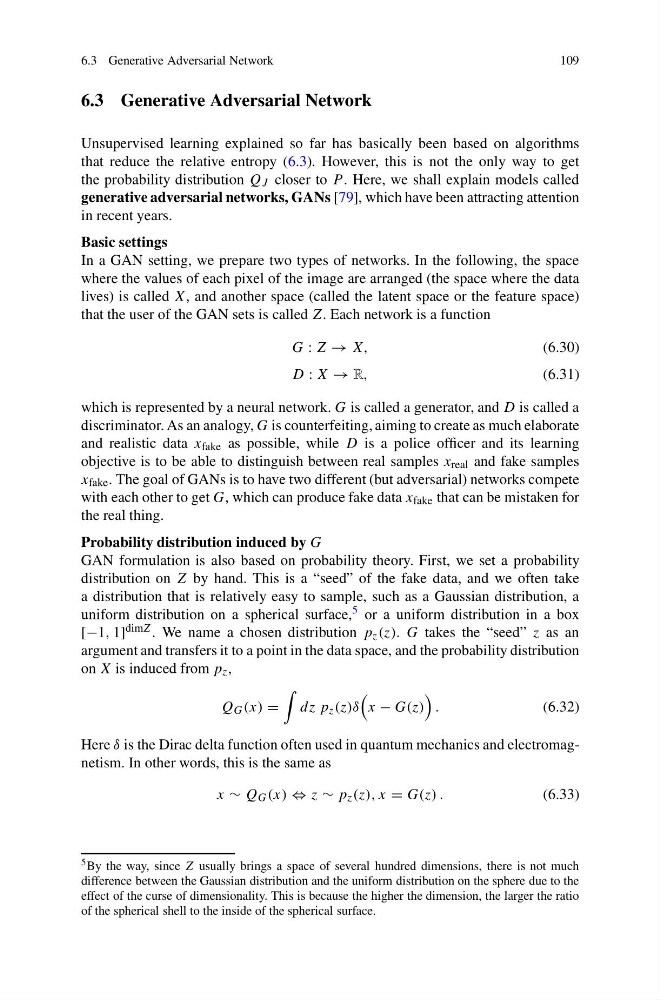
6.3 Generative Adversarial Network
109
6.3 Generative Adversarial Network
Unsupervised learning explained so far has basically been based on algorithms
that reduce the relative entropy (6.3). However, this is not the only way to get
the probability distribution Q J closer to P . Here, we shall explain models called
generative adversarial networks, GANs [79], which have been attracting attention
in recent years.
Basic settings
In a GAN setting, we prepare two types of networks. In the following, the space
where the values of each pixel of the image are arranged (the space where the data
lives) is called X, and another space (called the latent space or the feature space)
that the user of the GAN sets is called Z. Each network is a function
G : Z → X,
(6.30)
D : X → R,
(6.31)
which is represented by a neural network. G is called a generator, and D is called a
discriminator. As an analogy, G is counterfeiting, aiming to create as much elaborate
and realistic data x fake as possible, while D is a police officer and its learning
objective is to be able to distinguish between real samples x real and fake samples
x fake . The goal of GANs is to have two different (but adversarial) networks compete
with each other to get G, which can produce fake data x fake that can be mistaken for
the real thing.
Probability distribution induced by G
GAN formulation is also based on probability theory. First, we set a probability
distribution on Z by hand. This is a “seed” of the fake data, and we often take
a distribution that is relatively easy to sample, such as a Gaussian distribution, a
uniform distribution on a spherical surface, 5 or a uniform distribution in a box
[−1, 1] dimZ . We name a chosen distribution p z (z). G takes the “seed” z as an
argument and transfers it to a point in the data space, and the probability distribution
on X is induced from p z ,
Q G (x) =
dz p z (z)δ
x − G(z)
.
(6.32)
Here δ is the Dirac delta function often used in quantum mechanics and electromagnetism. In other words, this is the same as
x ∼ Q G (x) ⇔ z ∼ p z (z), x = G(z) .
(6.33)
5 By the way, since Z usually brings a space of several hundred dimensions, there is not much
difference between the Gaussian distribution and the uniform distribution on the sphere due to the
effect of the curse of dimensionality. This is because the higher the dimension, the larger the ratio
of the spherical shell to the inside of the spherical surface.
109
6.3 Generative Adversarial Network
Unsupervised learning explained so far has basically been based on algorithms
that reduce the relative entropy (6.3). However, this is not the only way to get
the probability distribution Q J closer to P . Here, we shall explain models called
generative adversarial networks, GANs [79], which have been attracting attention
in recent years.
Basic settings
In a GAN setting, we prepare two types of networks. In the following, the space
where the values of each pixel of the image are arranged (the space where the data
lives) is called X, and another space (called the latent space or the feature space)
that the user of the GAN sets is called Z. Each network is a function
G : Z → X,
(6.30)
D : X → R,
(6.31)
which is represented by a neural network. G is called a generator, and D is called a
discriminator. As an analogy, G is counterfeiting, aiming to create as much elaborate
and realistic data x fake as possible, while D is a police officer and its learning
objective is to be able to distinguish between real samples x real and fake samples
x fake . The goal of GANs is to have two different (but adversarial) networks compete
with each other to get G, which can produce fake data x fake that can be mistaken for
the real thing.
Probability distribution induced by G
GAN formulation is also based on probability theory. First, we set a probability
distribution on Z by hand. This is a “seed” of the fake data, and we often take
a distribution that is relatively easy to sample, such as a Gaussian distribution, a
uniform distribution on a spherical surface, 5 or a uniform distribution in a box
[−1, 1] dimZ . We name a chosen distribution p z (z). G takes the “seed” z as an
argument and transfers it to a point in the data space, and the probability distribution
on X is induced from p z ,
Q G (x) =
dz p z (z)δ
x − G(z)
.
(6.32)
Here δ is the Dirac delta function often used in quantum mechanics and electromagnetism. In other words, this is the same as
x ∼ Q G (x) ⇔ z ∼ p z (z), x = G(z) .
(6.33)
5 By the way, since Z usually brings a space of several hundred dimensions, there is not much
difference between the Gaussian distribution and the uniform distribution on the sphere due to the
effect of the curse of dimensionality. This is because the higher the dimension, the larger the ratio
of the spherical shell to the inside of the spherical surface.