

100
5 Sampling
i, j is a symbol that indicates that the sum is taken for the nearest neighbor pairs
of the lattice points.
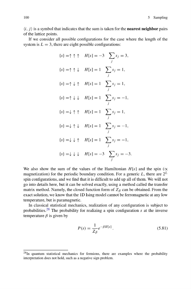
If we consider all possible configurations for the case where the length of the
system is L = 3, there are eight possible configurations:
{s} =↑ ↑ ↑ H [s] = −3
j
s j = 3,
{s} =↑ ↑ ↓ H [s] = 1
j
s j = 1,
{s} =↑ ↓ ↑ H [s] = 1
j
s j = 1,
{s} =↑ ↓ ↓ H [s] = 1
j
s j = −1,
{s} =↓ ↑ ↑ H [s] = 1
j
s j = 1,
{s} =↓ ↑ ↓ H [s] = 1
j
s j = −1,
{s} =↓ ↓ ↑ H [s] = 1
j
s j = −1,
{s} =↓ ↓ ↓ H [s] = −3
j
s j = −3.
We also show the sum of the values of the Hamiltonian H [s] and the spin (∝
magnetization) for the periodic boundary condition. For a generic L, there are 2 L
spin configurations, and we find that it is difficult to add up all of them. We will not
go into details here, but it can be solved exactly, using a method called the transfer
matrix method. Namely, the closed function form of Z β can be obtained. From the
exact solution, we know that the 1D Ising model cannot be ferromagnetic at any low
temperature, but is paramagnetic.
In classical statistical mechanics, realization of any configuration is subject to
probabilities. 28 The probability for realizing a spin configuration s at the inverse
temperature β is given by
P (s) =
1
Z β
e
−βH [s] .
(5.81)
28 In quantum statistical mechanics for fermions, there are examples where the probability
interpretation does not hold, such as a negative sign problem.
5 Sampling
i, j is a symbol that indicates that the sum is taken for the nearest neighbor pairs
of the lattice points.
If we consider all possible configurations for the case where the length of the
system is L = 3, there are eight possible configurations:
{s} =↑ ↑ ↑ H [s] = −3
j
s j = 3,
{s} =↑ ↑ ↓ H [s] = 1
j
s j = 1,
{s} =↑ ↓ ↑ H [s] = 1
j
s j = 1,
{s} =↑ ↓ ↓ H [s] = 1
j
s j = −1,
{s} =↓ ↑ ↑ H [s] = 1
j
s j = 1,
{s} =↓ ↑ ↓ H [s] = 1
j
s j = −1,
{s} =↓ ↓ ↑ H [s] = 1
j
s j = −1,
{s} =↓ ↓ ↓ H [s] = −3
j
s j = −3.
We also show the sum of the values of the Hamiltonian H [s] and the spin (∝
magnetization) for the periodic boundary condition. For a generic L, there are 2 L
spin configurations, and we find that it is difficult to add up all of them. We will not
go into details here, but it can be solved exactly, using a method called the transfer
matrix method. Namely, the closed function form of Z β can be obtained. From the
exact solution, we know that the 1D Ising model cannot be ferromagnetic at any low
temperature, but is paramagnetic.
In classical statistical mechanics, realization of any configuration is subject to
probabilities. 28 The probability for realizing a spin configuration s at the inverse
temperature β is given by
P (s) =
1
Z β
e
−βH [s] .
(5.81)
28 In quantum statistical mechanics for fermions, there are examples where the probability
interpretation does not hold, such as a negative sign problem.