

Column: From Ising Model to Hopfield Model
101
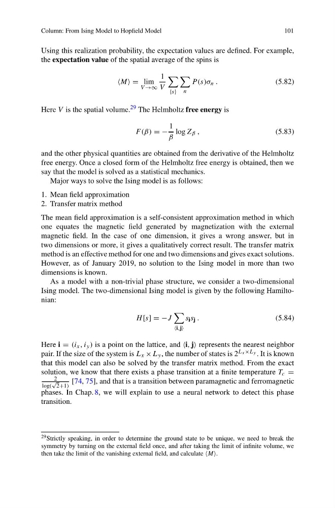
Using this realization probability, the expectation values are defined. For example,
the expectation value of the spatial average of the spins is
M = lim
V →∞
1
V
{s}
n
P (s)σ n .
(5.82)
Here V is the spatial volume. 29 The Helmholtz free energy is
F (β) = −
1
β
log Z β ,
(5.83)
and the other physical quantities are obtained from the derivative of the Helmholtz
free energy. Once a closed form of the Helmholtz free energy is obtained, then we
say that the model is solved as a statistical mechanics.
Major ways to solve the Ising model is as follows:
1. Mean field approximation
2. Transfer matrix method
The mean field approximation is a self-consistent approximation method in which
one equates the magnetic field generated by magnetization with the external
magnetic field. In the case of one dimension, it gives a wrong answer, but in
two dimensions or more, it gives a qualitatively correct result. The transfer matrix
method is an effective method for one and two dimensions and gives exact solutions.
However, as of January 2019, no solution to the Ising model in more than two
dimensions is known.
As a model with a non-trivial phase structure, we consider a two-dimensional
Ising model. The two-dimensional Ising model is given by the following Hamiltonian:
H [s] = −J
i,j
s i s j .
(5.84)
Here i = (i x , i y ) is a point on the lattice, and i, j represents the nearest neighbor
pair. If the size of the system is L x × L y , the number of states is 2 L x ×L y . It is known
that this model can also be solved by the transfer matrix method. From the exact
solution, we know that there exists a phase transition at a finite temperature T c =
2
log(
√
2+1)
[74, 75], and that is a transition between paramagnetic and ferromagnetic
phases. In Chap. 8, we will explain to use a neural network to detect this phase
transition.
29 Strictly speaking, in order to determine the ground state to be unique, we need to break the
symmetry by turning on the external field once, and after taking the limit of infinite volume, we
then take the limit of the vanishing external field, and calculate M.
101
Using this realization probability, the expectation values are defined. For example,
the expectation value of the spatial average of the spins is
M = lim
V →∞
1
V
{s}
n
P (s)σ n .
(5.82)
Here V is the spatial volume. 29 The Helmholtz free energy is
F (β) = −
1
β
log Z β ,
(5.83)
and the other physical quantities are obtained from the derivative of the Helmholtz
free energy. Once a closed form of the Helmholtz free energy is obtained, then we
say that the model is solved as a statistical mechanics.
Major ways to solve the Ising model is as follows:
1. Mean field approximation
2. Transfer matrix method
The mean field approximation is a self-consistent approximation method in which
one equates the magnetic field generated by magnetization with the external
magnetic field. In the case of one dimension, it gives a wrong answer, but in
two dimensions or more, it gives a qualitatively correct result. The transfer matrix
method is an effective method for one and two dimensions and gives exact solutions.
However, as of January 2019, no solution to the Ising model in more than two
dimensions is known.
As a model with a non-trivial phase structure, we consider a two-dimensional
Ising model. The two-dimensional Ising model is given by the following Hamiltonian:
H [s] = −J
i,j
s i s j .
(5.84)
Here i = (i x , i y ) is a point on the lattice, and i, j represents the nearest neighbor
pair. If the size of the system is L x × L y , the number of states is 2 L x ×L y . It is known
that this model can also be solved by the transfer matrix method. From the exact
solution, we know that there exists a phase transition at a finite temperature T c =
2
log(
√
2+1)
[74, 75], and that is a transition between paramagnetic and ferromagnetic
phases. In Chap. 8, we will explain to use a neural network to detect this phase
transition.
29 Strictly speaking, in order to determine the ground state to be unique, we need to break the
symmetry by turning on the external field once, and after taking the limit of infinite volume, we
then take the limit of the vanishing external field, and calculate M.