

Column: From Ising Model to Hopfield Model
99
This is the heatbath method for the Ising model. We see that the spins other than the
spin of our focus are considered as a heatbath and fixed. Also, thanks to focusing on
one site, we have only two states, and the denominator of the transition probability
can be calculated. We perform this for each point and update the whole. 26 However,
because of this framework, it is not always possible to use the heatbath method for
general models.
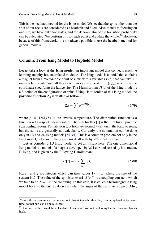
Column: From Ising Model to Hopfield Model
Let us take a look at the Ising model, an important model that connects machine
learning and physics, and related models. 27 The Ising model is a model that explains
a magnet from a microscopic point of view, with a variable (spin) that can take ±1
on each lattice site. We call this a configuration and write s = {s n } n , where n is the
coordinate specifying the lattice site. The Hamiltonian H [s] of the Ising model is
a function of the configuration of spins. Using Hamiltonian of this Ising model, the
partition function Z β is written as follows:
Z β =
{s}
e
−βH [s] ,
(5.79)
where β = 1/(k B T ) is the inverse temperature. The distribution function is a
function with respect to temperature. The sum for this {s} is the sum for all possible
spin configurations. Distribution functions are formally written in the form of sums,
but the sums are generally not calculable. Currently, the summation can be done
only in 1D and 2D Ising models [74, 75]. This is a common problem not only in the
Ising model, but also in many systems dealt with by statistical mechanics.
Let us consider a 1D Ising model to get an insight here. The one-dimensional
Ising model is a model of a magnet developed by W. Lenz and solved by his student,
E. Ising, and is given by the following Hamiltonian:
H [s] = −J
i,j
s i s j .
(5.80)
Here i and j are integers which can take values 1 · · · , L, where the size of the
system is L. The value of the spin is s i = ±1. J (>0) is a coupling constant, which
we take to be J = 1 in the following. In this case, it is called a ferromagnetic Ising
model because the energy decreases when the signs of the spins are aligned. Also,
26 Since the even-numbered points are not closest to each other, they can be updated at the same
time, so that part can be parallelized.
27 Here, we use the formulation of statistical mechanics without explaining the statistical mechanics
itself.
99
This is the heatbath method for the Ising model. We see that the spins other than the
spin of our focus are considered as a heatbath and fixed. Also, thanks to focusing on
one site, we have only two states, and the denominator of the transition probability
can be calculated. We perform this for each point and update the whole. 26 However,
because of this framework, it is not always possible to use the heatbath method for
general models.
Column: From Ising Model to Hopfield Model
Let us take a look at the Ising model, an important model that connects machine
learning and physics, and related models. 27 The Ising model is a model that explains
a magnet from a microscopic point of view, with a variable (spin) that can take ±1
on each lattice site. We call this a configuration and write s = {s n } n , where n is the
coordinate specifying the lattice site. The Hamiltonian H [s] of the Ising model is
a function of the configuration of spins. Using Hamiltonian of this Ising model, the
partition function Z β is written as follows:
Z β =
{s}
e
−βH [s] ,
(5.79)
where β = 1/(k B T ) is the inverse temperature. The distribution function is a
function with respect to temperature. The sum for this {s} is the sum for all possible
spin configurations. Distribution functions are formally written in the form of sums,
but the sums are generally not calculable. Currently, the summation can be done
only in 1D and 2D Ising models [74, 75]. This is a common problem not only in the
Ising model, but also in many systems dealt with by statistical mechanics.
Let us consider a 1D Ising model to get an insight here. The one-dimensional
Ising model is a model of a magnet developed by W. Lenz and solved by his student,
E. Ising, and is given by the following Hamiltonian:
H [s] = −J
i,j
s i s j .
(5.80)
Here i and j are integers which can take values 1 · · · , L, where the size of the
system is L. The value of the spin is s i = ±1. J (>0) is a coupling constant, which
we take to be J = 1 in the following. In this case, it is called a ferromagnetic Ising
model because the energy decreases when the signs of the spins are aligned. Also,
26 Since the even-numbered points are not closest to each other, they can be updated at the same
time, so that part can be parallelized.
27 Here, we use the formulation of statistical mechanics without explaining the statistical mechanics
itself.