

45
DGov
t axcredit
fueltax
0
10
0 4
I
I
I
W
=
´
-
(
)
.
,
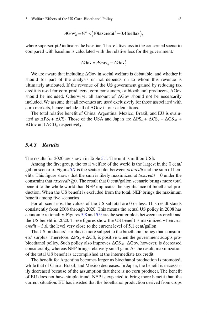
where superscript I indicates the baseline. The relative loss in the concerned scenario
compared with baseline is calculated with the relative loss for the government:
D
D
D
Gov
Gov
Gov
=
-
0
0
I
We are aware that including ∆Gov in social welfare is debatable, and whether it
should for part of the analysis or not depends on to whom this revenue is
ultimately attributed. If the revenue of the US government gained by reducing tax
credit is used for corn producers, corn consumers, or bioethanol producers, ∆Gov
should be included. Otherwise, all amount of ∆Gov should not be necessarily
included. We assume that all revenues are used exclusively for those associated with
corn markets, hence include all of ∆Gov in our calculations.
The total relative benefit of China, Argentina, Mexico, Brazil, and EU is evaluated as ΔPS i + ΔCS i . Those of the USA and Japan are ΔPS u + ΔCS u + ΔCS eth +
ΔGov and ∆CD j , respectively.
5.4.3 Results
The results for 2020 are shown in Table 5.1. The unit is million US$.
Among the first group, the total welfare of the world is the largest in the 0 cent/
gallon scenario. Figure 5.7 is the scatter plot between taxcredit and the sum of benefits. This figure shows that the sum is likely maximized at taxcredit = 0 under the
constraint that taxcredit ≧0. The result that 0 cent/gallon scenario brings more total
benefit to the whole world than NEP implicates the significance of bioethanol production. When the US benefit is excluded from the total, NEP brings the maximum
benefit among five scenarios.
For all scenarios, the values of the US subtotal are 0 or less. This result stands
consistently from 2008 through 2020. This means the actual US policy in 2008 has
economic rationality. Figures 5.8 and 5.9 are the scatter plots between tax credit and
the US benefit in 2020. These figures show the US benefit is maximized when taxcredit = 3.6, the level very close to the current level of 5.1 cent/gallon.
The US producers’ surplus is more subject to the bioethanol policy than consumers’ surplus. Therefore, ΔPS u + ΔCS u is positive when the government adopts probioethanol policy. Such policy also improves ∆CS eth . ∆Gov, however, is decreased
considerably, whereas NEP brings relatively small gain. As the result, maximization
of the total US benefit is accomplished at the intermediate tax credit.
The benefit for Argentina becomes larger as bioethanol production is promoted,
while that of China, Brazil, and Mexico decreases. In Japan, the benefit is necessarily decreased because of the assumption that there is no corn producer. The benefit
of EU does not have simple trend. NEP is expected to bring more benefit than the
current situation. EU has insisted that the bioethanol production derived from crops
5 Welfare Effects of the US Corn-Bioethanol Policy
DGov
t axcredit
fueltax
0
10
0 4
I
I
I
W
=
´
-
(
)
.
,
where superscript I indicates the baseline. The relative loss in the concerned scenario
compared with baseline is calculated with the relative loss for the government:
D
D
D
Gov
Gov
Gov
=
-
0
0
I
We are aware that including ∆Gov in social welfare is debatable, and whether it
should for part of the analysis or not depends on to whom this revenue is
ultimately attributed. If the revenue of the US government gained by reducing tax
credit is used for corn producers, corn consumers, or bioethanol producers, ∆Gov
should be included. Otherwise, all amount of ∆Gov should not be necessarily
included. We assume that all revenues are used exclusively for those associated with
corn markets, hence include all of ∆Gov in our calculations.
The total relative benefit of China, Argentina, Mexico, Brazil, and EU is evaluated as ΔPS i + ΔCS i . Those of the USA and Japan are ΔPS u + ΔCS u + ΔCS eth +
ΔGov and ∆CD j , respectively.
5.4.3 Results
The results for 2020 are shown in Table 5.1. The unit is million US$.
Among the first group, the total welfare of the world is the largest in the 0 cent/
gallon scenario. Figure 5.7 is the scatter plot between taxcredit and the sum of benefits. This figure shows that the sum is likely maximized at taxcredit = 0 under the
constraint that taxcredit ≧0. The result that 0 cent/gallon scenario brings more total
benefit to the whole world than NEP implicates the significance of bioethanol production. When the US benefit is excluded from the total, NEP brings the maximum
benefit among five scenarios.
For all scenarios, the values of the US subtotal are 0 or less. This result stands
consistently from 2008 through 2020. This means the actual US policy in 2008 has
economic rationality. Figures 5.8 and 5.9 are the scatter plots between tax credit and
the US benefit in 2020. These figures show the US benefit is maximized when taxcredit = 3.6, the level very close to the current level of 5.1 cent/gallon.
The US producers’ surplus is more subject to the bioethanol policy than consumers’ surplus. Therefore, ΔPS u + ΔCS u is positive when the government adopts probioethanol policy. Such policy also improves ∆CS eth . ∆Gov, however, is decreased
considerably, whereas NEP brings relatively small gain. As the result, maximization
of the total US benefit is accomplished at the intermediate tax credit.
The benefit for Argentina becomes larger as bioethanol production is promoted,
while that of China, Brazil, and Mexico decreases. In Japan, the benefit is necessarily decreased because of the assumption that there is no corn producer. The benefit
of EU does not have simple trend. NEP is expected to bring more benefit than the
current situation. EU has insisted that the bioethanol production derived from crops
5 Welfare Effects of the US Corn-Bioethanol Policy