

44
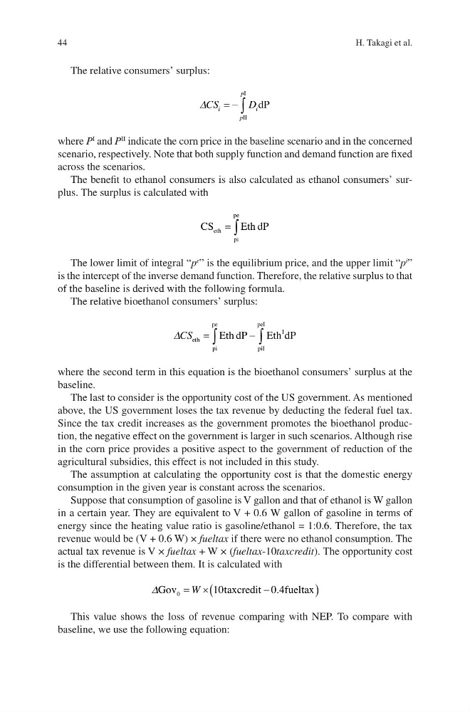
The relative consumers’ surplus:
DCS
D
i
p
p
i
= - ò
II
I
dP
where P
I
and P
II
indicate the corn price in the baseline scenario and in the concerned
scenario, respectively. Note that both supply function and demand function are fixed
across the scenarios.
The benefit to ethanol consumers is also calculated as ethanol consumers’ surplus. The surplus is calculated with
CS
Eth dP
eth
pi
pe
= ò
The lower limit of integral “p
e
” is the equilibrium price, and the upper limit “p
i
”
is the intercept of the inverse demand function. Therefore, the relative surplus to that
of the baseline is derived with the following formula.
The relative bioethanol consumers’ surplus:
DCS eth
pi
pe
piI
peI
I
Eth dP
Eth dP
=
-
ò
ò
where the second term in this equation is the bioethanol consumers’ surplus at the
baseline.
The last to consider is the opportunity cost of the US government. As mentioned
above, the US government loses the tax revenue by deducting the federal fuel tax.
Since the tax credit increases as the government promotes the bioethanol production, the negative effect on the government is larger in such scenarios. Although rise
in the corn price provides a positive aspect to the government of reduction of the
agricultural subsidies, this effect is not included in this study.
The assumption at calculating the opportunity cost is that the domestic energy
consumption in the given year is constant across the scenarios.
Suppose that consumption of gasoline is V gallon and that of ethanol is W gallon
in a certain year. They are equivalent to V + 0.6 W gallon of gasoline in terms of
energy since the heating value ratio is gasoline/ethanol = 1:0.6. Therefore, the tax
revenue would be (V + 0.6 W) × fueltax if there were no ethanol consumption. The
actual tax revenue is V × fueltax + W × (fueltax-10taxcredit). The opportunity cost
is the differential between them. It is calculated with
DGov
t axcredit
fueltax
0
10
0 4
= ´
-
(
)
W
.
This value shows the loss of revenue comparing with NEP. To compare with
baseline, we use the following equation:
H. Takagi et al.
The relative consumers’ surplus:
DCS
D
i
p
p
i
= - ò
II
I
dP
where P
I
and P
II
indicate the corn price in the baseline scenario and in the concerned
scenario, respectively. Note that both supply function and demand function are fixed
across the scenarios.
The benefit to ethanol consumers is also calculated as ethanol consumers’ surplus. The surplus is calculated with
CS
Eth dP
eth
pi
pe
= ò
The lower limit of integral “p
e
” is the equilibrium price, and the upper limit “p
i
”
is the intercept of the inverse demand function. Therefore, the relative surplus to that
of the baseline is derived with the following formula.
The relative bioethanol consumers’ surplus:
DCS eth
pi
pe
piI
peI
I
Eth dP
Eth dP
=
-
ò
ò
where the second term in this equation is the bioethanol consumers’ surplus at the
baseline.
The last to consider is the opportunity cost of the US government. As mentioned
above, the US government loses the tax revenue by deducting the federal fuel tax.
Since the tax credit increases as the government promotes the bioethanol production, the negative effect on the government is larger in such scenarios. Although rise
in the corn price provides a positive aspect to the government of reduction of the
agricultural subsidies, this effect is not included in this study.
The assumption at calculating the opportunity cost is that the domestic energy
consumption in the given year is constant across the scenarios.
Suppose that consumption of gasoline is V gallon and that of ethanol is W gallon
in a certain year. They are equivalent to V + 0.6 W gallon of gasoline in terms of
energy since the heating value ratio is gasoline/ethanol = 1:0.6. Therefore, the tax
revenue would be (V + 0.6 W) × fueltax if there were no ethanol consumption. The
actual tax revenue is V × fueltax + W × (fueltax-10taxcredit). The opportunity cost
is the differential between them. It is calculated with
DGov
t axcredit
fueltax
0
10
0 4
= ´
-
(
)
W
.
This value shows the loss of revenue comparing with NEP. To compare with
baseline, we use the following equation:
H. Takagi et al.