

40
Scenario 5:
P
P
% P
%
E10
2 7 20
80 12
=
´
+
´
( )
¢
/ .
gas
Scenario 6:
Eth Pop
Pdif
/
.
.
.
= -
+
´
´
+
´
´
(
) ´ ( )
¢¢
-
-
0 00530 5 50 10
267 10
2 7
6
6
T
P
P
% P
%
E10
2 7 20
80 12
=
´
+
´
( )
²
/ .
gas
5.3.3 Results
Figure 5.5 shows the simulation results of corn price in the first group along with
the actual values from 1991 to 2006. In all scenarios, the price goes downward. This
is especially remarkable in NEP. In all scenarios but NEP, the price settles in the
range of 200–300 cent/bushel, the level at which price has actually stayed for more
than 30 years.
Expanding demand for corn is met mainly through growing yield. The US corn
yield was 9.5 t/ha in 2007 and is expected to be 10.8 t/ha in 2020. Harvested area
does not expand so much in any scenario. In 18.4 cent/gallon scenario which needs
the largest area of all scenarios tested, it is expected to be 32.3 million ha in 2020.
Although it exceeds the maximum area recorded prior to the simulation’s initial year
(30.4 million ha in 1985), the difference is not so large relative to its amplitude.
In 2008, the actual corn price jumped up to 497.5 cent/bushel (USDA/ERS
n.d.-a). One of the causes was bioethanol production. Because crude oil price in
2008 was $97.26/bbl (BP n.d.), bioethanol consumption must have been promoted.
Then, how much impact did the rise in crude oil price have on corn price? We simulated corn price in 2008 by setting crude oil price at the actual value.
The results show that the calculated corn price in 2008 is no more than 257.7
cent/bushel. Even when replacing $97.26/bbl with $147/bbl (the highest crude oil
price in 2008), calculated corn price is only 306.8 cent/bushel. The most likely reason for such a surprising result is that a rise in crude oil price brings not only a
higher gasoline price but a higher E10 price.
9
1
E10
E20
8
2
Bioethanol
Gasoline
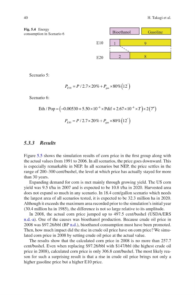
Fig. 5.4 Energy
consumption in Scenario 6
H. Takagi et al.
Scenario 5:
P
P
% P
%
E10
2 7 20
80 12
=
´
+
´
( )
¢
/ .
gas
Scenario 6:
Eth Pop
Pdif
/
.
.
.
= -
+
´
´
+
´
´
(
) ´ ( )
¢¢
-
-
0 00530 5 50 10
267 10
2 7
6
6
T
P
P
% P
%
E10
2 7 20
80 12
=
´
+
´
( )
²
/ .
gas
5.3.3 Results
Figure 5.5 shows the simulation results of corn price in the first group along with
the actual values from 1991 to 2006. In all scenarios, the price goes downward. This
is especially remarkable in NEP. In all scenarios but NEP, the price settles in the
range of 200–300 cent/bushel, the level at which price has actually stayed for more
than 30 years.
Expanding demand for corn is met mainly through growing yield. The US corn
yield was 9.5 t/ha in 2007 and is expected to be 10.8 t/ha in 2020. Harvested area
does not expand so much in any scenario. In 18.4 cent/gallon scenario which needs
the largest area of all scenarios tested, it is expected to be 32.3 million ha in 2020.
Although it exceeds the maximum area recorded prior to the simulation’s initial year
(30.4 million ha in 1985), the difference is not so large relative to its amplitude.
In 2008, the actual corn price jumped up to 497.5 cent/bushel (USDA/ERS
n.d.-a). One of the causes was bioethanol production. Because crude oil price in
2008 was $97.26/bbl (BP n.d.), bioethanol consumption must have been promoted.
Then, how much impact did the rise in crude oil price have on corn price? We simulated corn price in 2008 by setting crude oil price at the actual value.
The results show that the calculated corn price in 2008 is no more than 257.7
cent/bushel. Even when replacing $97.26/bbl with $147/bbl (the highest crude oil
price in 2008), calculated corn price is only 306.8 cent/bushel. The most likely reason for such a surprising result is that a rise in crude oil price brings not only a
higher gasoline price but a higher E10 price.
9
1
E10
E20
8
2
Bioethanol
Gasoline
Fig. 5.4 Energy
consumption in Scenario 6
H. Takagi et al.