

86
3 Investigation of Euler–Bernoulli Beams in the Elastic Range
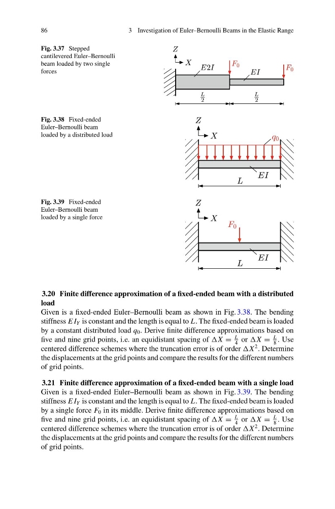
Fig. 3.37 Stepped
cantilevered Euler–Bernoulli
beam loaded by two single
forces
Fig. 3.38 Fixed-ended
Euler–Bernoulli beam
loaded by a distributed load
Fig. 3.39 Fixed-ended
Euler–Bernoulli beam
loaded by a single force
3.20 Finite difference approximation of a fixed-ended beam with a distributed
load
Given is a fixed-ended Euler–Bernoulli beam as shown in Fig. 3.38. The bending
stiffness E I Y is constant and the length is equal to L. The fixed-ended beam is loaded
by a constant distributed load q 0 . Derive finite difference approximations based on
five and nine grid points, i.e. an equidistant spacing of =
L
4
or =
L
8
. Use
centered difference schemes where the truncation error is of order
2 . Determine
the displacements at the grid points and compare the results for the different numbers
of grid points.
3.21 Finite difference approximation of a fixed-ended beam with a single load
Given is a fixed-ended Euler–Bernoulli beam as shown in Fig. 3.39. The bending
stiffness E I Y is constant and the length is equal to L. The fixed-ended beam is loaded
by a single force F 0 in its middle. Derive finite difference approximations based on
five and nine grid points, i.e. an equidistant spacing of =
L
4
or =
L
8
. Use
centered difference schemes where the truncation error is of order
2 . Determine
the displacements at the grid points and compare the results for the different numbers
of grid points.
3 Investigation of Euler–Bernoulli Beams in the Elastic Range
Fig. 3.37 Stepped
cantilevered Euler–Bernoulli
beam loaded by two single
forces
Fig. 3.38 Fixed-ended
Euler–Bernoulli beam
loaded by a distributed load
Fig. 3.39 Fixed-ended
Euler–Bernoulli beam
loaded by a single force
3.20 Finite difference approximation of a fixed-ended beam with a distributed
load
Given is a fixed-ended Euler–Bernoulli beam as shown in Fig. 3.38. The bending
stiffness E I Y is constant and the length is equal to L. The fixed-ended beam is loaded
by a constant distributed load q 0 . Derive finite difference approximations based on
five and nine grid points, i.e. an equidistant spacing of =
L
4
or =
L
8
. Use
centered difference schemes where the truncation error is of order
2 . Determine
the displacements at the grid points and compare the results for the different numbers
of grid points.
3.21 Finite difference approximation of a fixed-ended beam with a single load
Given is a fixed-ended Euler–Bernoulli beam as shown in Fig. 3.39. The bending
stiffness E I Y is constant and the length is equal to L. The fixed-ended beam is loaded
by a single force F 0 in its middle. Derive finite difference approximations based on
five and nine grid points, i.e. an equidistant spacing of =
L
4
or =
L
8
. Use
centered difference schemes where the truncation error is of order
2 . Determine
the displacements at the grid points and compare the results for the different numbers
of grid points.