

3.5 Supplementary Problems
85
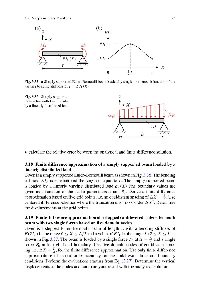
Fig. 3.35 a Simply supported Euler–Bernoulli beam loaded by single moments; b function of the
varying bending stiffness E I Y = E I Y (X )
Fig. 3.36 Simply supported
Euler–Bernoulli beam loaded
by a linearly distributed load
• calculate the relative error between the analytical and finite difference solution.
3.18 Finite difference approximation of a simply supported beam loaded by a
linearly distributed load
Given is a simply supported Euler–Bernoulli beam as shown in Fig. 3.36. The bending
stiffness E I Y is constant and the length is equal to L. The simply supported beam
is loaded by a linearly varying distributed load q Z (X ) (the boundary values are
given as a function of the scalar parameters α and β). Derive a finite difference
approximation based on five grid points, i.e. an equidistant spacing of =
L
4
. Use
centered difference schemes where the truncation error is of order
2 . Determine
the displacements at the grid points.
3.19 Finite difference approximation of a stepped cantilevered Euler–Bernoulli
beam with two single forces based on five domain nodes
Given is a stepped Euler–Bernoulli beam of length L with a bending stiffness of
E(2I Y ) in the range 0 ≤ X ≤ L/2 and a value of E I Y in the range L/2 ≤ X ≤ L as
shown in Fig. 3.37. The beam is loaded by a single force F 0 at X =
L
2
and a single
force F 0 at its right-hand boundary. Use five domain nodes of equidistant spacing, i.e. =
L
4
, for the finite difference approximation. Use only finite difference
approximations of second-order accuracy for the nodal evaluations and boundary
conditions. Perform the evaluations starting from Eq. (3.27). Determine the vertical
displacements at the nodes and compare your result with the analytical solution.
85
Fig. 3.35 a Simply supported Euler–Bernoulli beam loaded by single moments; b function of the
varying bending stiffness E I Y = E I Y (X )
Fig. 3.36 Simply supported
Euler–Bernoulli beam loaded
by a linearly distributed load
• calculate the relative error between the analytical and finite difference solution.
3.18 Finite difference approximation of a simply supported beam loaded by a
linearly distributed load
Given is a simply supported Euler–Bernoulli beam as shown in Fig. 3.36. The bending
stiffness E I Y is constant and the length is equal to L. The simply supported beam
is loaded by a linearly varying distributed load q Z (X ) (the boundary values are
given as a function of the scalar parameters α and β). Derive a finite difference
approximation based on five grid points, i.e. an equidistant spacing of =
L
4
. Use
centered difference schemes where the truncation error is of order
2 . Determine
the displacements at the grid points.
3.19 Finite difference approximation of a stepped cantilevered Euler–Bernoulli
beam with two single forces based on five domain nodes
Given is a stepped Euler–Bernoulli beam of length L with a bending stiffness of
E(2I Y ) in the range 0 ≤ X ≤ L/2 and a value of E I Y in the range L/2 ≤ X ≤ L as
shown in Fig. 3.37. The beam is loaded by a single force F 0 at X =
L
2
and a single
force F 0 at its right-hand boundary. Use five domain nodes of equidistant spacing, i.e. =
L
4
, for the finite difference approximation. Use only finite difference
approximations of second-order accuracy for the nodal evaluations and boundary
conditions. Perform the evaluations starting from Eq. (3.27). Determine the vertical
displacements at the nodes and compare your result with the analytical solution.