

3.4 Solved Problems
79
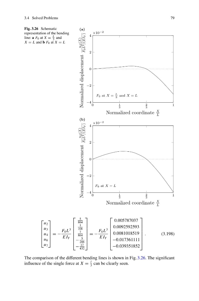
Fig. 3.26 Schematic
representation of the bending
line: a F 0 at X =
L
3 and
X = L and b F 0 at X = L
(a)
0
1
3
2
3
1
−4
−2
0
2
4
×10
−2
F0 at X =
L
3
and X = L
Normalized coordinate
X
L
Normalized displacement
u
Z (X)
F
0 L 3
/(EI
Y )
(b)
0
1
3
2
3
1
−4
−2
0
2
4
×10
−2
F0 at X = L
Normalized coordinate
X
L
Normalized displacement
u
Z (X)
F
0 L 3
/(EI
Y )
⎡
⎢
⎢
⎢
⎢
⎣
u 2
u 3
u 4
u 6
u 7
⎤
⎥
⎥
⎥
⎥
⎦
= −
F 0 L
3
E I Y
⎡
⎢
⎢
⎢
⎢
⎢
⎢
⎣
5
864
1
108
7
864
−
5
288
−
17
432
⎤
⎥
⎥
⎥
⎥
⎥
⎥
⎦
= −
F 0 L
3
E I Y
⎡
⎢
⎢
⎢
⎢
⎢
⎢
⎣
0.005787037
0.0092592593
0.0081018519
−0.017361111
−0.039351852
⎤
⎥
⎥
⎥
⎥
⎥
⎥
⎦
.
(3.198)
The comparison of the different bending lines is shown in Fig. 3.26. The significant
influence of the single force at X =
l
3
can be clearly seen.
79
Fig. 3.26 Schematic
representation of the bending
line: a F 0 at X =
L
3 and
X = L and b F 0 at X = L
(a)
0
1
3
2
3
1
−4
−2
0
2
4
×10
−2
F0 at X =
L
3
and X = L
Normalized coordinate
X
L
Normalized displacement
u
Z (X)
F
0 L 3
/(EI
Y )
(b)
0
1
3
2
3
1
−4
−2
0
2
4
×10
−2
F0 at X = L
Normalized coordinate
X
L
Normalized displacement
u
Z (X)
F
0 L 3
/(EI
Y )
⎡
⎢
⎢
⎢
⎢
⎣
u 2
u 3
u 4
u 6
u 7
⎤
⎥
⎥
⎥
⎥
⎦
= −
F 0 L
3
E I Y
⎡
⎢
⎢
⎢
⎢
⎢
⎢
⎣
5
864
1
108
7
864
−
5
288
−
17
432
⎤
⎥
⎥
⎥
⎥
⎥
⎥
⎦
= −
F 0 L
3
E I Y
⎡
⎢
⎢
⎢
⎢
⎢
⎢
⎣
0.005787037
0.0092592593
0.0081018519
−0.017361111
−0.039351852
⎤
⎥
⎥
⎥
⎥
⎥
⎥
⎦
.
(3.198)
The comparison of the different bending lines is shown in Fig. 3.26. The significant
influence of the single force at X =
l
3
can be clearly seen.