

78
3 Investigation of Euler–Bernoulli Beams in the Elastic Range
⎡
⎢
⎢
⎢
⎢
⎣
u 2
u 3
u 4
u 6
u 7
⎤
⎥
⎥
⎥
⎥
⎦
= −
F 0 L
3
E I Y
⎡
⎢
⎢
⎢
⎢
⎢
⎢
⎣
1
864
1
432
1
288
−
11
864
−
13
432
⎤
⎥
⎥
⎥
⎥
⎥
⎥
⎦
= −
F 0 L
3
E I Y
⎡
⎢
⎢
⎢
⎢
⎢
⎢
⎣
0.0011574074
0.0023148148
0.0034722222
−0.012731481
−0.030092593
⎤
⎥
⎥
⎥
⎥
⎥
⎥
⎦
.
(3.189)
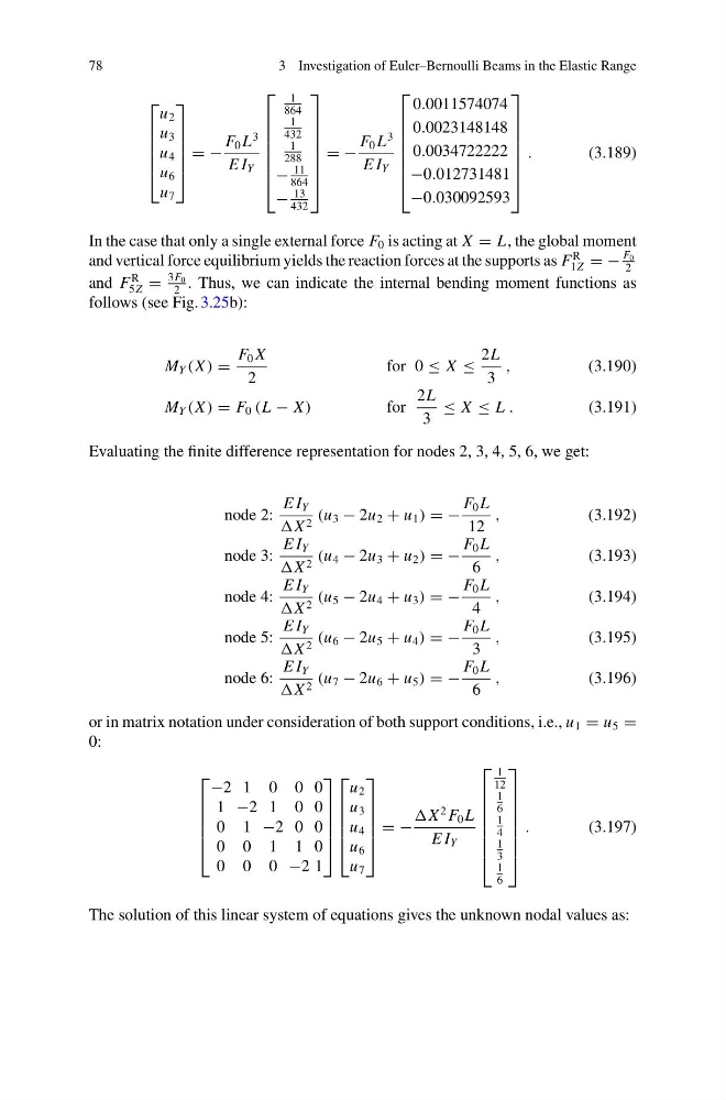
In the case that only a single external force F 0 is acting at X = L, the global moment
and vertical force equilibrium yields the reaction forces at the supports as F
R
1Z = −
F 0
2
and F
R
5Z =
3F 0
2
. Thus, we can indicate the internal bending moment functions as
follows (see Fig. 3.25b):
M Y (X ) =
F 0 X
2
for 0 ≤ X ≤
2L
3
,
(3.190)
M Y (X ) = F 0 (L − X )
for
2L
3
≤ X ≤ L .
(3.191)
Evaluating the finite difference representation for nodes 2, 3, 4, 5, 6, we get:
node 2:
E I Y
X 2 (u 3 − 2u 2 + u 1 ) = −
F 0 L
12
,
(3.192)
node 3:
E I Y
X 2 (u 4 − 2u 3 + u 2 ) = −
F 0 L
6
,
(3.193)
node 4:
E I Y
X 2 (u 5 − 2u 4 + u 3 ) = −
F 0 L
4
,
(3.194)
node 5:
E I Y
X 2 (u 6 − 2u 5 + u 4 ) = −
F 0 L
3
,
(3.195)
node 6:
E I Y
X 2 (u 7 − 2u 6 + u 5 ) = −
F 0 L
6
,
(3.196)
or in matrix notation under consideration of both support conditions, i.e., u 1 = u 5 =
0:
⎡
⎢
⎢
⎢
⎢
⎣
−2 1 0 0 0
1 −2 1 0 0
0 1 −2 0 0
0 0 1 1 0
0 0 0 −2 1
⎤
⎥
⎥
⎥
⎥
⎦
⎡
⎢
⎢
⎢
⎢
⎣
u 2
u 3
u 4
u 6
u 7
⎤
⎥
⎥
⎥
⎥
⎦
= −
X
2 F 0 L
E I Y
⎡
⎢
⎢
⎢
⎢
⎢
⎢
⎣
1
12
1
6
1
4
1
3
1
6
⎤
⎥
⎥
⎥
⎥
⎥
⎥
⎦
.
(3.197)
The solution of this linear system of equations gives the unknown nodal values as:
3 Investigation of Euler–Bernoulli Beams in the Elastic Range
⎡
⎢
⎢
⎢
⎢
⎣
u 2
u 3
u 4
u 6
u 7
⎤
⎥
⎥
⎥
⎥
⎦
= −
F 0 L
3
E I Y
⎡
⎢
⎢
⎢
⎢
⎢
⎢
⎣
1
864
1
432
1
288
−
11
864
−
13
432
⎤
⎥
⎥
⎥
⎥
⎥
⎥
⎦
= −
F 0 L
3
E I Y
⎡
⎢
⎢
⎢
⎢
⎢
⎢
⎣
0.0011574074
0.0023148148
0.0034722222
−0.012731481
−0.030092593
⎤
⎥
⎥
⎥
⎥
⎥
⎥
⎦
.
(3.189)
In the case that only a single external force F 0 is acting at X = L, the global moment
and vertical force equilibrium yields the reaction forces at the supports as F
R
1Z = −
F 0
2
and F
R
5Z =
3F 0
2
. Thus, we can indicate the internal bending moment functions as
follows (see Fig. 3.25b):
M Y (X ) =
F 0 X
2
for 0 ≤ X ≤
2L
3
,
(3.190)
M Y (X ) = F 0 (L − X )
for
2L
3
≤ X ≤ L .
(3.191)
Evaluating the finite difference representation for nodes 2, 3, 4, 5, 6, we get:
node 2:
E I Y
X 2 (u 3 − 2u 2 + u 1 ) = −
F 0 L
12
,
(3.192)
node 3:
E I Y
X 2 (u 4 − 2u 3 + u 2 ) = −
F 0 L
6
,
(3.193)
node 4:
E I Y
X 2 (u 5 − 2u 4 + u 3 ) = −
F 0 L
4
,
(3.194)
node 5:
E I Y
X 2 (u 6 − 2u 5 + u 4 ) = −
F 0 L
3
,
(3.195)
node 6:
E I Y
X 2 (u 7 − 2u 6 + u 5 ) = −
F 0 L
6
,
(3.196)
or in matrix notation under consideration of both support conditions, i.e., u 1 = u 5 =
0:
⎡
⎢
⎢
⎢
⎢
⎣
−2 1 0 0 0
1 −2 1 0 0
0 1 −2 0 0
0 0 1 1 0
0 0 0 −2 1
⎤
⎥
⎥
⎥
⎥
⎦
⎡
⎢
⎢
⎢
⎢
⎣
u 2
u 3
u 4
u 6
u 7
⎤
⎥
⎥
⎥
⎥
⎦
= −
X
2 F 0 L
E I Y
⎡
⎢
⎢
⎢
⎢
⎢
⎢
⎣
1
12
1
6
1
4
1
3
1
6
⎤
⎥
⎥
⎥
⎥
⎥
⎥
⎦
.
(3.197)
The solution of this linear system of equations gives the unknown nodal values as: